How Focal Statistics works
Available with Image Server
Focal Statistics performs an operation that calculates a statistic for input cells within a set of overlapping windows or neighborhoods. The statistic (for example, mean, maximum, or sum) is calculated for all input cells contained within each neighborhood.
Neighborhood processing
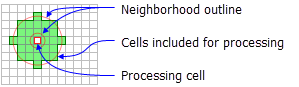
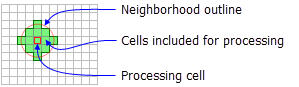
Conceptually, the algorithm visits each cell in the input raster and calculates a statistic for the cells that fall in the specified neighborhood shape around it. The cell for which the statistic is being calculated is referred to as the processing cell. The value of the processing cell is typically included in the neighborhood statistics calculation, but depending on the shape of the neighborhood, it might not be. Since neighborhoods will overlap in the scan process, input cells that are included in the calculation for one processing cell may also contribute in the calculation for another processing cell.
Several predefined neighborhood shapes available to choose from. You can also create a custom shape. The statistics that you can calculate for a neighborhood are majority, maximum, mean, median, minimum, minority, percentile, range, standard deviation, sum, and variety.
Example calculation
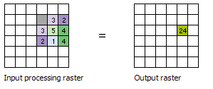
To illustrate the neighborhood processing for Focal Statistics, consider calculating a Sum statistic of the neighborhood around the processing cell with the value of 5 in the following diagram. A rectangular 3 by 3 cell neighborhood shape is specified and the Ignore NoData in calculations parameter is left at the default checked setting. The sum of the values of the neighboring cells (3 + 2 + 3 + 4 + 2 + 1 + 4 = 19) plus the value of the processing cell (5) equals 24 (19 + 5 = 24). A value of 24 is given to the cell in the output raster in the same location as the processing cell in the input raster.
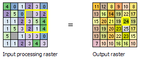
The above diagram demonstrates how the calculations are performed on a single cell in the input raster. In the following diagram, the results for all the input cells are shown. The cells highlighted in yellow identify the same processing cell and neighborhood as in the example above.
NoData cells
The Ignore NoData in calculations parameter controls how NoData cells within the neighborhood window are processed. When this parameter is checked (ignore_nodata = "DATA" in Python), any cells in the neighborhood that are NoData will be ignored in the calculation of the output value for the processing cell. When unchecked (ignore_nodata = "NODATA" in Python), if any cell in the neighborhood is NoData, the output value for the processing cell will be NoData.
If the processing cell itself is NoData, with the Ignore NoData in calculations option selected, the output value for the cell will be calculated based on the other cells in the neighborhood that have a valid value. If all of the cells in the neighborhood are NoData, the output will be NoData.
Corner and edge cells
When the processing cell is near the corners and edges of the input raster, the number of cells that are included in the neighbourhood is adjusted accordingly. The calculation of the statistic is also adjusted.
The following diagrams illustrate how the output statistic is calculated for each processing cell from the available cells in each individual neighborhood. The process starts at the upper left corner of the input raster and scans from left to right across each row before proceeding to the next row. The neighborhood used in this example is a 3 by 3 cell rectangle, and the statistic used is sum. The Ignore NoData in calculations parameter is left at the default checked setting. In the diagrams, the neighborhood is outlined in yellow, and the processing cell is outlined in cyan.
For the first processing cell, because it is at upper left corner of the input raster 6 by 6 cell raster, there are only four cells available to be in the neighborhood. Adding those values together results in the output value for the first cell being assigned a value of 11. For the next cell to the right, there are now six cells in the neighborhood, and the sum is calculated for those. The scan proceeds across all the cells in the first row. To save space, not all the processing cells are shown.
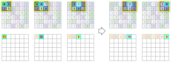
Note that in the first row, for the third processing cell from the left (value = 1), one of the input cells has a value of NoData. Because the tool was set to ignore NoData, that particular cell will be ignored in the calculations. If the statistic to be calculated had been set to Mean instead of Sum, it would be calculated as the sum of all the cells in the neighborhood that are not NoData, divided by 5.
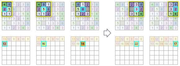
For the second row of input cells, the statistic for the first processing cell will be calculated based on having six cells available in the neighborhood. For the next processing cell, there will be nine cells to consider in the calculation. For the subsequent cell, there will be eight input values to calculate with, since one of the cells in the 3 by 3 neighborhood is NoData. The process continues for the rest of the cells in the row and then on to the following rows until all the processing cells have been analyzed.
Neighborhood size and performance
The tool can process very large neighborhoods. However, as the neighborhood increases in size, the performance will be impacted since more input cells will be included in each calculation. The rectangle neighborhood type has some optimizations that allow for increased performance relative to other neighbourhood shapes for a given area.
The maximum size of any dimension of a neighborhood is limited to 4,096 cells. This means that rectangular neighborhoods cannot exceed this number of cells in either the horizontal or vertical direction. For circular neighborhoods, the radius cannot exceed 2,047 cells.
Neighborhood types
The shape of a neighborhood can be an annulus (a donut), a circle, a rectangle, or a wedge. Using a kernel file, you can also define a custom neighborhood shape, as well as assign different weights to specific cells in the neighborhood before the statistic is calculated.
Following are descriptions of the neighborhood shapes and how they are defined:
Annulus
The annulus shape is composed of two circles, one inside the other to make a donut shape. Cells with centers that fall outside the radius of the smaller circle but inside the radius of the larger circle will be included in processing the neighborhood. The area that falls between the two circles constitutes the annulus neighborhood.
The radius is identified in cells or map units, measured perpendicular to the x- or y-axis. When the radii are specified in map units, they are converted to radii in cell units. The resulting radii in cell units produce an area that most closely represents the area calculated using the original radii in map units. Any cell center encompassed by the annulus will be included in the processing of the neighborhood.
The default annulus neighborhood is an inner radius of one cell and an outer radius of three cells.
An example illustration of an annulus neighborhood follows:
A processing cell with the default annulus neighborhood (inner radius = 1 cell, outer radius = 3 cells). Circle
A circle neighborhood is created by specifying a radius value.
The radius is identified in cell or map units, measured perpendicular to the x- or y-axis. When the radius is specified in map units, additional logic is used to determine which cells are included in the processing neighborhood. First, the exact area of a circle defined by the specified radius value is calculated. Next, the area is calculated for two additional circles, one with the specified radius value rounded down and one with the specified radius value rounded up. These two areas are compared to the result from the specified radius, and the radius of the area that is closest will be used in the operation.
The default circle neighborhood radius is three cells.
An example illustration of a circle neighborhood follows:
A processing cell with a circle neighborhood (radius = 2 cells). Rectangle
The rectangle neighborhood is specified by providing a width and a height in either cells or map units.
Only the cells with centers that fall within the defined object are processed as part of the rectangle neighborhood.
The default rectangle neighborhood is a square with a height and width of three cells.
The x,y position for the processing cell within the neighborhood, with respect to the upper left corner of the neighborhood, is determined by the following equations:
\[ \]
\begin{align*} x \space = \space (width \space of \space the \space neighborhood \space + \space 1)/2 \y \space = \space (height \space of \space the \space neighborhood \space + \space 1)/2 \end{align*}
If the input number of cells is even, the x- and y-coordinates are computed using truncation.
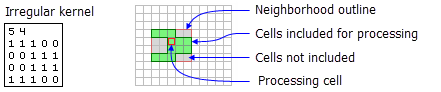
The following apply to a kernel file for an irregular neighborhood:
The irregular kernel file is an ASCII text file that defines the values and shape of an irregular neighborhood. The file can be created with any plain text editor. It must have a
.txtfile extension and no spaces in the file name.The first line specifies the width and height of the neighborhood (the number of cells in the x direction, followed by a space, and the number of cells in the y direction).
The subsequent lines define the value to use for each position in the neighborhood they represent. A space between each value is necessary.
The values define whether a position in the neighborhood will be included in the calculation. Typically, the value 1 is used to identify the positions to include in the calculations for an irregular neighbourhood, but any positive or negative value other than 0 can be used. Floating point values can also be used.
To exclude a location in the neighborhood from the calculation, use a value of 0 (not a blank space) at the corresponding location in the kernel file.
The following example shows the contents of an irregular kernel file and the neighborhood it represents:
Weight
Similar to the irregular neighborhood type, the weight neighborhood allows you to define an irregular neighborhood around the processing cell but also allows you to apply weights to the input values.
The weight kernel file specifies the cell positions to include within the neighborhood and the weights by which they will be multiplied.
The weight neighborhood is only available for the mean, standard deviation, and sum statistics types.
The x,y position for the processing cell within the neighborhood, with respect to the upper left corner of the neighborhood, is determined by the following equations:
\[ \]
\begin{align*} x \space = \space (width \space + \space 1)/2 \y \space = \space (height \space + \space 1)/2 \end{align*}
\begin{align*} 4 \space 6 \space 7 \6 \space 7 \space 8 \4 \space 5 \space 6 \end{align*}
\begin{align*} 3 \space 3 \0.0 \space 0.5 \space 0.0 \space \0.5 \space 2.0 \space 0.5 \space \0.0 \space 0.5 \space 0.0 \end{align*}
\begin{align*} = \space ( \textit _{1} \textit _{1} \space + \space \textit _{2} \textit _{2} \space + \space \textit _{3} \textit _{3} \space + \space \textit _{4} \textit _{4} \space + \space \textit _{5} \textit _{5} \space + \space \textit _{6} \textit _{6} \space + \space \textit _{7} \textit _{7} \space + \space \textit _{8} \textit _{8} \space + \space w _{9} \textit _{9} ) \space / \ \space \space ( \textit _{1} \space + \space \textit _{2} \space + \space \textit _{3} \space + \space \textit _{4} \space + \space \textit _{5} \space + \space \textit _{6} \space + \space \textit _{7} \space + \space \textit _{8} \space + \space \textit _{9} ) \= \space ((0 * 4)+(0.5 * 6)+(0 * 7)+(0.5 * 6)+(2.0 * 7)+(0.5 * 8)+(0 * 4)+(0.5 * 5)+(0 * 6)) \space / \ \space \space (0 \space + \space 0.5 \space + \space 0 \space + \space 0.5 \space + \space 2.0 \space + \space 0.5 \space + \space 0 \space + \space 0.5 \space + \space 0) \= \space (0 \space + \space 3.0 \space + \space 0 \space + \space 3.0 \space + \space 14.0 \space + \space 4.0 \space + \space 0 \space + \space 2.5 \space + \space 0) \space / \space \ \space \space (0.5 \space + \space 0.5 \space + \space 2.0 \space + \space 0.5 \space + \space 0.5) \= \space (3.0 \space + \space 3.0 \space + \space 14.0 \space + \space 4.0 \space + \space 2.5) \space / \space 4.0 \= \space 26.5 \space / \space 4.0 \= \space 6.625 \end{align*}
\begin{align*} 4 \space 6 \space 7 \6 \space 7 \space 8 \4 \space 5 \space 6 \end{align*}
\begin{align*} 3 \space 3 \0.0 \space 0.5 \space 0.0 \space \0.5 \space 2.0 \space 0.5 \space \0.0 \space 0.5 \space 0.0 \end{align*}
\begin{align*} 4 \space 6 \space 7 \6 \space 7 \space 8 \4 \space 5 \space 6 \end{align*}
\begin{align*} 3 \space 3 \-1 \space -2 \space -1 \ \space 0 \space \space 0 \space \space 0 \ \space 1 \space \space 2 \space \space 1 \end{align*}
\begin{align*} = \space ( \textit _{1} \textit _{1} \space + \space \textit _{2} \textit _{2} \space + \space \textit _{3} \textit _{3} \space + \space \textit _{4} \textit _{4} \space + \space \textit _{5} \textit _{5} \space + \space \textit _{6} \textit _{6} \space + \space \textit _{7} \textit _{7} \space + \space \textit _{8} \textit _{8} \space + \space \textit _{9} \textit _{9} ) \= \space ((-1 * 4) \space + \space (-2 * 6) \space + \space (-1 * 7) \space + \space (0 * 6) \space + \space (0 * 7) \space + \space (0 * 8) \space + \space (1 * 4) \space + \space (2 * 5) \space + \space (1 * 6)) \= \space (-4) \space + \space (-12) \space + \space (-7) \space + \space 4 \space + \space 10 \space + \space 6 \= \space -3 \ \end{align*}