How Probabilistic Kernel Density works
 Available with the Spatial Analyst license.
The Probabilistic Kernel Density tool estimates the density of point features while quantifying the uncertainty of that estimate. The tool repeats the estimate specified amount of times under one or more sources of uncertainty. It differs from traditional density analysis because it treats the inputs as uncertain. Rather than generating a single density estimate, it repeatedly recalculates density while accounting for uncertainty in point weights, point locations, or the sampled set of points. The tool then summarizes the simulation results into a mean density surface and uncertainty measures that describe the variability of the estimate. This allows you to evaluate not only where density is high, but also how confident you can be in that result.
Benefits of Probabilistic Kernel Density
The Probabilistic Kernel Density tool combines kernel density estimation with simulation-based uncertainty propagation (Heuvelink, 1998). Compared to a traditional density estimate, it offers the following benefits:
Produces a mean density surface and can optionally generate standard deviation, coefficient of variation, and exceedance probability rasters. These outputs help quantify uncertainty in the density estimate.
Distinguishes stable density patterns from patterns driven by a small number of uncertain observations. This can support more informed decision-making.
Identifies which concentrations are stable and which are artifacts of a few uncertain points, supporting more defensible decisions.
Provides flexibility for modeling uncertainty. You can configure the uncertainty type, sampling method, sampling strategy, attribute error model, and distribution method to match your data and analytical requirements.
Calculate probabilistic kernel density
Conceptually, the tool fits a smooth kernel surface over each point, similar to the Kernel Density tool. The kernel surface is based on the quartic kernel function described in Silverman (1986, p. 76).
For each output cell, the density value is calculated as the sum of all kernel surface values at the center of that cell with the following formula:
where:
\(\large \hat{\lambda}_h(s)\) is the estimated density at location \(s\) using bandwidth \(h\).
\(n\) is the number of event points.
\(w_i\) is the weight of event \(i\), where \(w_i = 1\) when no Population Field parameter value is specified. It will be
NONEby default.\(h\) is the bandwidth (search radius) in map units.
\(K\) is the kernel function.
\(\large |s-x_i|\) is the distance from location \(s\) to event \(i\).
The Probabilistic Kernel Density tool extends this estimate through simulation. For each simulation, the inputs are randomly adjusted to reflect the selected sources of uncertainty These adjustments, referred to as perturbations, may affect point locations, point weights, or the sampled set of points before a kernel density surface is calculated. After all simulations are complete, the resulting surfaces are summarized to generate the output rasters.
Output density value from a single simulation is calculated using the following formula:
where:
\(\hat{\lambda}^{b}_h(s)\) is the estimated density at location \(s\) using bandwidth \(h\) in simulation \(b\).
\(n_b\) is the number of points used in simulation \(b\) (equal to \(n\) unless subsampling is used).
\(w_i^{(b)}\) is the weight of point \(i\) in simulation \(b\) after attribute perturbation.
\(x_i^{(b)}\) is the location of point \(i\) in simulation \(b\) after any location perturbation.
\(h\) is the bandwidth (search radius) in map units.
\(K\) is the kernel function.
\(\large |s-x_i^{b}|\) is the distance from location \(s\) to point \(i\) in simulation \(b\).
A single run proceeds in two stages. First, the simulation stage generates many density surfaces based on perturbed inputs. Then, the summary stage combines these surfaces to produce the output rasters.
Simulation stage
Each of the \(B\) simulations perturbs the inputs according to the selected uncertainty types and computes a kernel density surface from the perturbed inputs.
The three available Uncertainty Type parameter values described below can be used individually or in combination. When multiple options are selected, all corresponding perturbations are applied within each simulation.
Sampling: This type represents sampling uncertainty. The events are resampled, so each simulation uses a slightly different sample of events.
Location: This type represents positional uncertainty. Each event location is offset by a random amount drawn from a normal distribution. The standard deviation of the displacement is calculated as the Location Displacement Factor parameter value multiplied by the Search Radius parameter value.
Attribute: This type represents uncertainty in the population-field weights. Each weight is redrawn from a distribution whose spread is defined by either a margin of error or a fixed percentage.
Summary stage
After the simulations are complete, the tool has a set of density values for each output cell. These values represent the distribution of the density estimate at that location.
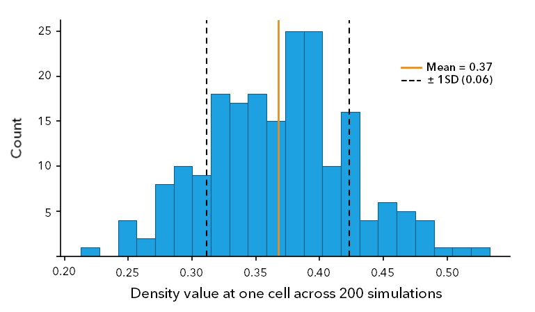
The mean of these values becomes the cell value in the primary density raster. Their variability becomes the cell values in the standard deviation and coefficient of variation output rasters. The exceedance probability raster records the proportion of simulated density values that exceed a specified threshold.
Because these summaries are calculated directly from the simulated values, no assumptions are made about the shape of the distribution.
The graph below shows an example of the distribution of simulated density values for a single cell. The mean density value becomes the cell value in the primary density raster, and the spread of the distribution is used to calculate the uncertainty rasters.
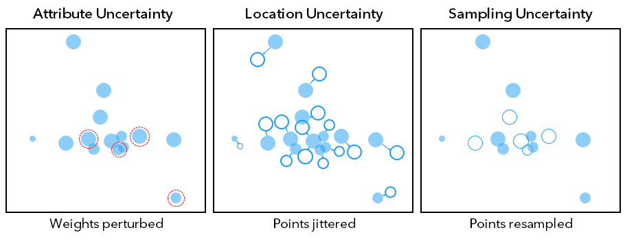
The three uncertainty types differ in what they perturb. The Attribute uncertainty type changes the weights, the Location uncertainty type changes the positions, and the Sampling uncertainty type changes the set of points used in the analysis.
The figure below illustrates the three uncertainty types available in the Probabilistic Kernel Density tool. Each uncertainty type modifies a different aspect of the input data during a simulation.
Sampling uncertainty
Sampling uncertainty represents the fact that the observed points are only a sample of the underlying population or process. A different sample could produce a different density surface. To account for this uncertainty, each simulation redraws the points using the selected Sampling Strategy and Sampling Method parameter values (Efron, 1979). The Percentage of Data to Sample parameter controls the size of the resampled dataset. The Sampling Strategy and Sampling Method parameters control how the resampling is performed.
Sampling strategy
The Sampling Strategy parameter determines how points are resampled. The strategies described below control how the resampled dataset is constructed.
Random sampling
This is the default sampling method. In each simulation, \(n\) points are drawn with replacements from the original set of \(N\) points (Efron, 1979). As a result, some points may be selected multiple times, while others may not be selected at all.
This approach provides an unbiased baseline. As the number of simulations increases, the sampling error decreases approximately in proportion to \(1 / \sqrt{B}\) (Metropolis and Ulam, 1949).
It applies the following formula:
\({\large \{x_i^{(b)}\}_{i=1}^{n}}\) ~ resample with replacement from \(\{x_1, \ldots, x_n\}\)
where:
\(x_i^{(b)}\) is the point drawn in simulation \(b\).
\(\{x_1, \ldots, x_n\}\) is the original set of points.
Tip:
Use the Random value for the Sampling Strategy parameter when sampling uncertainty is the primary focus. Because points are selected randomly, it provides an unbiased representation of how density estimates vary across simulations.
Subsampling
Subsampling draws a smaller set of \(m\) distinct points without replacement (Politis, Romano, and Wolf, 1999). The subsample size is determined by the Percentage of Data to Sample parameter.
The number of points selected for each simulation is calculated using the following formula:
\(\large m = \lfloor \ pn \ \rfloor\)
where:
\(m\) is the subsample size.
\(p\) is the fraction specified by the Percentage of Data to Sample parameter.
\(n\) is the number of input points.
The subsample for simulation \(b\) is then obtained by selecting \(m\) points at random without replacement from the original set of \(n\) points.
The subsample is represented by the following formula:
\(\large S^{(b)} \subset X, \qquad |S^{(b)}| = m\)
where:
\(S^{(b)}\) is the subsample selected for simulation \(b\).
\(m\) is the subsample size.
\(X\) is the full set of input points.
Tip:
Use the Subsampling value for the Sampling Strategy parameter when working with large datasets or when reducing clustering is important. By using a smaller subset of the data in each simulation, it can help evaluate the sensitivity of density estimates to sampling variation.
Farthest point sampling
Farthest point sampling selects points that are as far apart as possible. At each step, it adds the point whose nearest already-selected neighbor is most distant (Eldar et al., 1997) by applying the following formula:
\(\large x_{k+1} = \Large{\arg\max_{x \in X \setminus S_k} \min_{s \in S_k}} \large \|x - s\|\)
where:
\(S_k\) is the set of points selected after step \(k\).
\(X\) is the full set of points.
\(x_{k+1}\) is the next point selected, chosen to maximize its distance from the current selection.
Tip:
Use the Farthest point sampling value for the Sampling Strategy parameter to maximize spatial coverage and reduce clustering. Because point selection is nearly deterministic, it may underestimate sampling uncertainty.
Compare sampling uncertainty
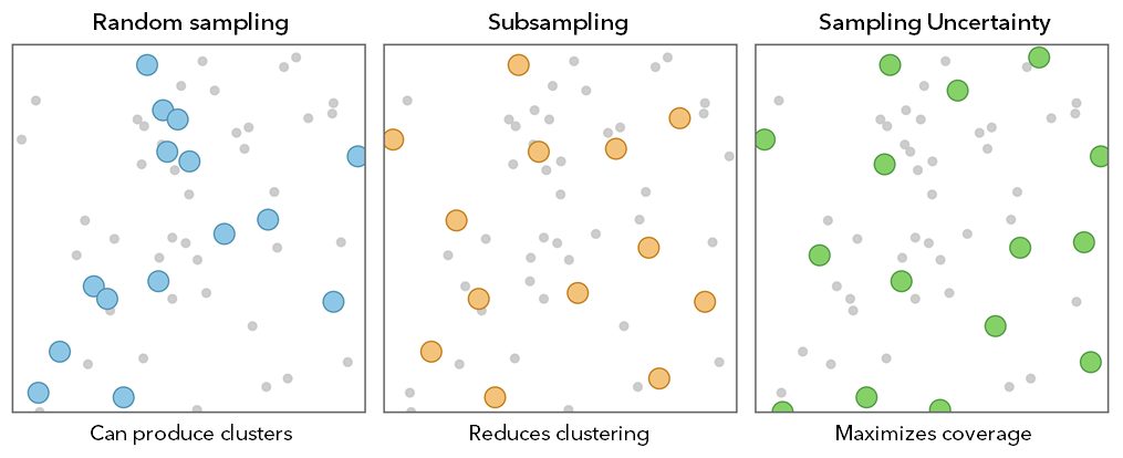
The figure below compares the three available Sampling Strategy options. Each strategy selects points differently, which affects the spatial pattern of the resampled dataset. Random sampling can produce clustered selections, subsampling reduces clustering by using fewer points, and farthest point sampling maximizes the spacing between selected points.
Sampling method
The Sampling Method parameter determines whether selected points are spatially adjusted after selection. The methods described below control how resampled points are positioned during each simulation.
Standard versus smooth bootstrap
The Sampling Method parameter controls whether resampled points remain at their original locations or are spatially adjusted. The Standard Bootstrap parameter option reuses the exact point locations. The Smooth Bootstrap parameter option adds a small kernel-shaped displacement to each resampled point (Silverman and Young, 1987). This adjustment helps reduce repeated placement of points at the same location. It can be particularly useful in sparse datasets, where a point selected multiple times would otherwise remain at exactly the same coordinates.
The displaced location of each resampled point is calculated using the following equation:
\(\Large{{x_i}^{*} = x_j + h_s \epsilon}\)
where:
\(x_i^{*}\) is the smoothed-bootstrap event location.
\(x_j\) is the resampled event location.
\(h_s\) is the kernel-noise bandwidth, proportional to \(h\).
\(\large \epsilon\) is the random displacement drawn from kernel \(K\).
Location uncertainty
Location uncertainty represents positional error in the points, such as a geocoded location, a GPS fix, or a centroid that is not exactly where the phenomenon is. Each simulation displaces every point by a random offset drawn from a bivariate normal distribution and re-estimates. The Location Displacement Factor parameter controls how far points are displaced, expressed as a fraction of the Search Radius value. Choose a value that reflects the positional accuracy of the input data.
Each point is displaced using the following equation:
\(\large{x_i^{*} = x_i + \delta_i}\)
where:
\(\delta_i\) is the random positional offset applied to event \(i\).
where:
\(\delta_i \sim N\left(0, \sigma^2 I_2\right)\)
It is a bivariate normal distribution with mean 0 and variance \(\sigma^2\) in each direction. The matrix \(I_2\) is the \(2 \times 2\) identity matrix.
\(\sigma\) is the positional error scale, calculated as the Location Displacement Factor value multiplied by \(h\).
\(x_i\) is the recorded location of event \(i\).
\(x_i^{*}\) is the displaced location of event \(i\).
For example, with a search radius of \(h = 1{,}000\) meters and a displacement factor of = 0.05, the offset scale is 50 meters. Each point is displaced by a random amount with a standard deviation of 50 meters in both directions before the surface is calculated.
Attribute uncertainty
Attribute uncertainty represents error in the weights specified using the Population field parameter. Each simulation redraws every weight from a probability distribution centered on the reported value. The perturbed weights preserve the original values as their mean and use the associated standard error to define the spread of the distribution by applying the following formulas:
where:
\(\mathbb{E}[w_i^{*}]\) is the mean of the perturbed weight, equal to the original.
\(\operatorname{Var}(w_i^*)\) is the variance of the perturbed weight.
\(w_i\) is the original weight of point \(i\).
\(SE_i\) is the standard error of the weight.
The Attribute Error Type parameter determines how the standard error is calculated. If a margin of error is available for each point, it is converted to a standard error using the confidence level specified by the Margin-of-Error Confidence Level parameter with the following formula:
\({MOE} = z \cdot SE, \quad SE = \large \frac{MOE}{z}\)
where:
\(MOE\) is the margin of error associated with a weight.
\(z\) is the critical value corresponding to the specified confidence level (1.645 for 90%, 1.960 for 95%, and 2.576 for 99%).
\(SE\) is the standard error associated with the weight.
The standard error can then be used to generate perturbed weights with the following formula:
\(w_i^{*} = w_i + SE_i \cdot Z, \quad Z \sim N(0, 1)\)
where:
\(w_i^{*}\) is the perturbed weight of event \(i\).
\(w_i\) is the original weight of event \(i\).
\(SE_i\) is the standard error of weight \(i\).
\(Z\) is a standard normal variable with mean 0 and variance 1.
If a margin of error is available for each point, the standard error can be derived from that margin of error. Alternatively, the Attribute Error Type parameter can be set to Fixed Percentage of Value, which calculates the standard error as a specified percentage of each weight with the following formula:
\(\large{SE_i = \frac{{attr\_error\_pct}}{100} \times w_i}\)
where:
\(SE_i\) is the standard error of weight \(i\).
\({attr\_error\_pct}\) is the assumed percentage error.
\(w_i\) is the original weight of event \(i\).
For example, a weight of 500 with a 95% margin of error of 98 gives \(SE = 98 / 1.960 = 50\). A fixed 10% error on the same weight gives \(SE = 0.10 \times 500 = 50\). The result achieves the same spread by a different route.
Distribution method
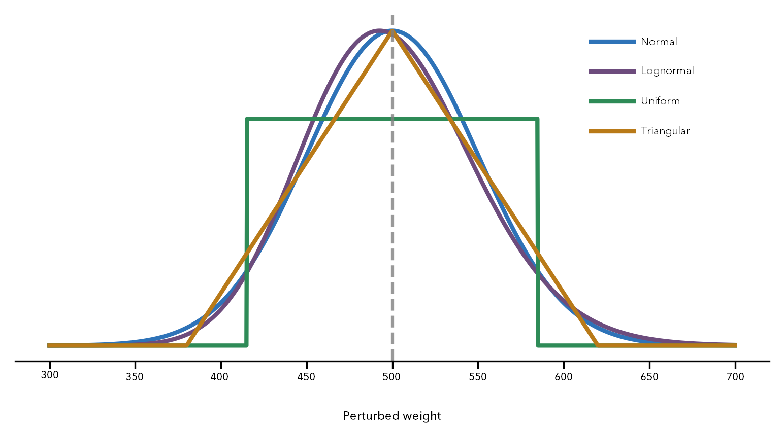
The Distribution Method parameter determines the probability distribution used to redraw the weights. All four methods are parameterized to preserve the same mean and the standard error. As a result, changing the distribution affects the shape of the uncertainty but not its overall magnitude.
The figure below compares the four Distribution Method options. All four distributions are parameterized to preserve the same mean and standard error. The distributions differ only in shape, which affects how uncertainty is distributed around the original weight.
Normal
The Normal distribution option redraws weights using a normal distribution centered on the original value.
The perturbed weight is calculated using the following formula:
\(w_i^{*} = w_i + SE_i \cdot Z, \quad Z \sim N(0, 1)\)
where:
\(w_i^{*}\) is the perturbed weight for event \(i\).
\(w_i\) is the original weight for event \(i\).
\(SE_i\) is the standard error of the weight.
\(Z\) is a standard normal random variable with mean 0 and variance 1.
For example, with \(w = 500\), \(SE = 50\), and \(Z = 1.2\), the perturbed weight is \(w^{*} = 500 + 1.2 \times 50 = 560\).
Lognormal
The Lognormal option is right-skewed and strictly positive, making it well suited for count data and other nonnegative quantities (Limpert, Stahel, and Abbt, 2001).
The perturbed weight is calculated using the following formula:
\(\large{w_i^{*} = w_i \times \exp\left(\sigma_{\ln} Z - \frac{1}{2}\sigma_{\ln}^2\right)}\)
where:
\(w_i^{*}\) is the perturbed weight for event \(i\)
\(w_i\) is the original weight for event \(i\)
\(\sigma_{\ln}\) is the lognormal shape parameter derived.
where \(\large{\sigma_{\ln} = \sqrt{\ln\left(1 + \left(\frac{SE_i}{w_i}\right)^2\right)}}\)
It is derived from \(SE_i\) and \(w_i\).
\(SE_i\) is the standard error of the weight
\(Z\) is a standard normal random variable with mean 0 and variance 1
For example, with \(w = 500\), \(SE = 50\), and \(Z = 1.2\), the lognormal shape parameter is \(\sigma_{\ln} = 0.0998\). The perturbed weight is \(w^{*} \approx 561\).
Uniform
The Uniform option draws weights from a symmetric interval centered on the original value. All values within the interval are equally likely.
The perturbed weight is calculated using the following formula:
\(\large{w_i^{*} \sim U(w_i - a_i,\; w_i + a_i), \quad a_i = 3SE_i}\)
where:
\(w_i^{*}\) is the perturbed weight for event \(i\).
\(w_i\) is the original weight for event \(i\).
\(SE_i\) is the standard error of the weight.
\(a_i\) is the half-width of the interval, equal to \(3SE_i\).
For example, with \(w = 500\) and \(SE = 50\), the half-width of the interval is \(a = 150\). The perturbed weight is drawn uniformly from \([350, 650]\). If a simulation draws 0.70 of the way across the interval, the perturbed weight is \(w^{*} = 350 + 0.70 \times (650 - 350) = 560\).
Triangular
The Triangular option draws weights from a symmetric triangular distribution centered on the original value. The original value is most likely, and the probability decreases linearly toward the limits.
The perturbed weight is calculated using the following formula:
\(\large{w_i^{*} \sim Tri(w_i - c_i,\; w_i + c_i), \quad c_i = \sqrt{6}\,SE_i}\)
where:
\(w_i^{*}\) is the perturbed weight for event \(i\).
\(w_i\) is the original weight for event \(i\).
\(SE_i\) is the standard error of the weight.
\(c_i\) is the half-width of the distribution, equal to \(\sqrt{6}\,SE_i\).
For example, with \(w = 500\) and \(SE = 50\), the half-width is \(c = \sqrt{6} \times 50 \approx 122.5\). The perturbed weight is drawn from a triangular distribution over the interval \([377.5, 622.5]\), with the highest probability at 500. One simulation might draw \(w^{*} = 560\).
Primary and additional output rasters
After the simulations finish, the tool has an ensemble of \(B\) density values at each cell. This ensemble represents the empirical distribution of the density estimate at that location. The output rasters summarize that ensemble. Because the summaries are calculated directly from the simulated values, no assumptions are made about the shape of the distribution.
Primary density raster
The Output Density Raster parameter value stores the summary of the simulated density values. The Output Density Calculation Method parameter value determines how those values are summarized for each cell.
The default Mean option returns the Monte Carlo estimate (Efron and Tibshirani, 1993). The Median, Minimum, and Maximum options return the corresponding summary statistic for each cell.
The Mean option calculates the primary density raster as follows:
\(\Large {\bar{\lambda}_s = \frac{1}{B}\sum_{b=1}^{B} \lambda_{b,s}}\)
where:
\(\bar{\lambda}_s\) is the mean density at cell \(s\).
\(B\) is the number of simulations.
\(b\) is the simulation index.
\(\lambda_{b,s}\) is the density at cell \(s\) in simulation \(b\).
Standard deviation raster
The Output Standard Deviation Raster parameter value stores the variability of the simulated density values. The standard deviation of the simulated density values at each cell is calculated using the following formula (Welford 1962):
\(\large{SD_s = \sqrt{\frac{1}{B-1}\sum_{b=1}^{B}(\lambda_{b,s} - \bar{\lambda}_s)^2}}\)
where:
\(SD_s\) is the standard deviation of density at cell \(s\).
\(\large \bar{\lambda}_s\) is the mean density at cell \(s\).
\(B\) is the number of simulations.
\(\large \lambda_{b,s}\) is the density at cell \(s\), repetition \(b\).
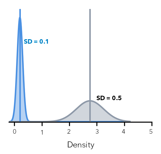
The figure below illustrates how standard deviation measures the spread of simulated density values. Although the distribution on the right has a larger mean density, it also has a larger standard deviation, indicating greater variability across simulations.
Coefficient of variation raster
The Output Coefficient of Variation Raster parameter value stores the variability of density relative to the mean density. To determine the coefficient of variation at each cell, the tool calculates the ratio of the standard deviation to the mean density using the following formula (Efron and Tibshirani, 1993):
\(\large CV_s = \LARGE \frac{SD_s}{\bar{\lambda}_s}\)
where:
\(CV_s\) is the coefficient of variation at cell \(s\).
\(SD_s\) is the standard deviation of density at cell \(s\).
\(\large \bar{\lambda}_s\) is the mean density at cell \(s\), with \(\large \bar{\lambda}_s \le 0\) treated as NoData.
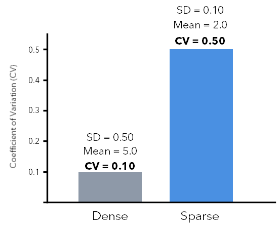
For example, a dense cell with a mean density of 5.0 and \(SD = 0.5\) has \(CV = 0.10\). A sparse cell with a mean density of 0.2 and \(SD = 0.1\) has \(CV = 0.50\). Although the sparse cell has a smaller standard deviation, its density estimate is more variable relative to its mean.
The figure below illustrates how the coefficient of variation (CV) measures variability relative to the mean density. Although the sparse cell has a smaller standard deviation, its density estimate has a higher coefficient of variation because the mean density is much lower.
Exceedance probability raster
The Output Exceedance Probability Raster parameter measures the probability that density exceeds a specified threshold at each cell. It is useful for identifying locations where density is consistently above a decision threshold across simulations (Efron and Tibshirani, 1993; Härdle and Marron, 1991).
The exceedance probability at each cell is calculated as the proportion of simulations whose density values exceed the specified threshold using the following formula:
\(\large P(\lambda_s > t) = \frac{1}{B}\sum_{b=1}^{B} \mathbf{1}(\lambda_{b,s} > t)\)
where:
\(P(\lambda_s > t)\) is the probability that density at cell \(s\) exceeds \(t\).
\(B\) is the number of simulations.
\(b\) is the simulation index.
\(\large \lambda_{b,s}\) is the density at cell \(s\) in simulation \(b\).
\(t\) is the probability threshold.
\(\mathbf{1}(\cdot)\) is the indicator function, equal to 1 when the condition is true and 0 otherwise.
The figure below illustrates how the exceedance probability raster is calculated. The probability is determined by comparing the simulated density values at a cell with a specified threshold and calculating the proportion of simulations that exceed that threshold.
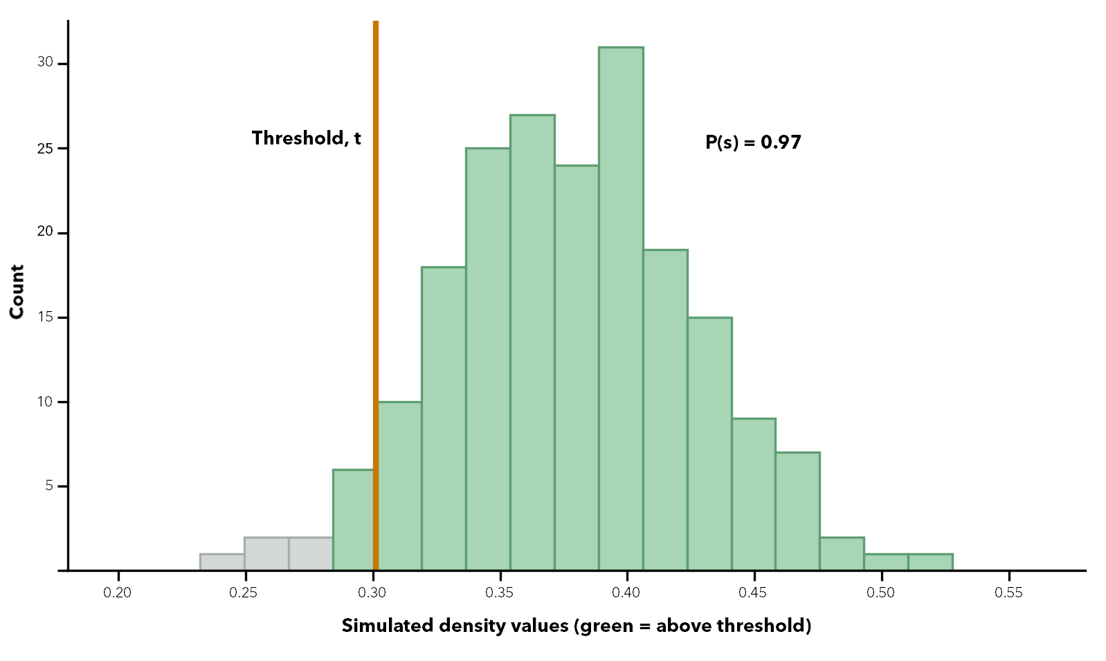
For example, if the 90th percentile of the mean surface is 0.30, then \(t = 0.30\). At a cell where 184 of 200 simulations exceeded 0.30, the exceedance probability is \(184 / 200 = 0.92\). At a cell where only 40 of 200 simulations exceed 0.30, the exceedance probability is \(40 / 200 = 0.20\). Increasing the threshold to the 95th percentile makes the exceedance criterion more stringent.
Effect of planar and geodesic methods on density
The calculation of output density values depends on the method used to measure distance. The Planar option of the Method parameter is appropriate for local analyses that use a projected coordinate system designed to preserve distance and area. By default, the tool uses a planar method.
The Geodesic option is appropriate for regional or global analyses, including analyses performed in a Web Mercator or geographic coordinate system. This method accounts for the curvature of the earth and correctly handles data near the poles and the international dateline.
Differences between planar and geodesic distance increase with geographic extent and distance from the source locations. For large study areas, the geodesic method is generally recommended.
Potential applications
The tool is useful when input data contains uncertainty and decisions depend on understanding its effects. The examples described below illustrate common applications.
Ecology and habitat
Species observations are often sparse and imprecise, and observation counts may also be uncertain. The Sampling, Location, and Attribute uncertainty types can reveal how sensitive density estimates are to observation coverage, positional error, and variability in reported counts.
Public safety
Incident locations and severity weights are often uncertain. The Location and Attribute uncertainty types can identify concentrations that remain consistent across simulations and distinguish them from less reliable concentrations.
Disease and health surveillance
Case counts, disease rates, and other health measures may include uncertainty from surveys or statistical models. The Attribute uncertainty type incorporates this uncertainty into the density estimate, helping identify areas where elevated risk is consistently supported across simulations.
Hazard and infrastructure exposure
Event counts and locations may both contain uncertainty. Combining uncertainty types and reviewing the exceedance probability raster can identify areas that consistently exceed a specified threshold across simulations.
Important considerations
The considerations described below can help with interpreting the outputs and understanding the effects of different parameter choices.
Multiple uncertainty types
When multiple uncertainty types are selected, their perturbations are applied together within each simulation. The reported uncertainty, therefore, reflects their combined effects rather than any single source. To evaluate the contribution of a specific uncertainty source, run the tool separately for each type, and compare the results.
Very large or very small population values
Very large or very small population values can influence the default search radius. If the default value produces unrealistic density patterns, consider specifying the search radius explicitly.
Too few simulations
The output rasters are estimates based on a finite number of simulations. Using too few simulations can produce unstable mean, standard deviation, and probability estimates. Increasing the number of simulations generally improves stability but increases processing time, particularly for the exceedance probability raster.
Choosing a distribution method
The Lognormal, Uniform, and Triangular distribution options for the Distribution Method parameter preserve the same mean and standard error but differ in shape. Lognormal is positively skewed and can produce occasional large values, while Uniform and Triangular are bounded and symmetric. For strictly positive quantities such as counts, select the distribution that best reflects the expected range and variability of the data.
Coefficient of variation near zero density
The coefficient of variation can become very large when mean density is close to zero. The tool assigns NoData to cells whose mean density is zero or less, but extreme values can still occur where mean density is very small. Interpret the coefficient of variation together with the mean density raster.
Interpreting the exceedance probability raster
The exceedance probability raster shows how often density exceeds the specified threshold across simulations. It does not represent the probability that an event occurs at a location. When reporting results, include the threshold or percentile used to generate the raster.
References
See the following references for additional information:
Efron, B. 1979. "Bootstrap Methods: Another Look at the Jackknife." Annals of Statistics 7, no. 1: 1–26.
Eldar, Y., M. Lindenbaum, M. Porat, and Y. Y. Zeevi. 1997. "The Farthest Point Strategy for Progressive Image Sampling." IEEE Transactions on Image Processing 6, no. 9: 1305–1315.
Heuvelink, G. B. M. 1998. Error Propagation in Environmental Modelling with GIS. London: Taylor & Francis.
Limpert, E., W. A. Stahel, and M. Abbt. 2001. "Log-normal Distributions across the Sciences: Keys and Clues." BioScience 51, no. 5: 341–352.
Politis, D. N., J. P. Romano, and M. Wolf. 1999. Subsampling. New York: Springer.
Silverman, B. W. 1986. Density Estimation for Statistics and Data Analysis. New York: Chapman and Hall.
Silverman, B. W., and G. A. Young. 1987. "The Bootstrap: To Smooth or Not to Smooth?" Biometrika 74, no. 3: 469–479.