How Top Hat Transform works
![]() Available with Spatial Analyst license.
Available with Spatial Analyst license.
The Top Hat Transform tool extracts spatial structures from an elevation surface. One way to use these extracted structures, such as valleys and water channels, is to validate the location of the hydrographic features in elevation-derived hydrography. The algorithm used by this tool is based on the top hat transformation function (Rodriguez, et al, 2002), using the input neighborhood as the structuring element.
The Analysis Type parameter controls which structures will be detected, ridges or valleys. At each cell location, the output value represents the height or depth of the spatial structure detected at that location.
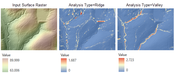
With the Ridge analysis type option, objects that are taller than their surroundings—such as dams and bridges—are highlighted. With the Valley analysis type option, objects that are lower than their surroundings—such as water channels—are highlighted.
Ridge analysis
The Ridge analysis type corresponds to the white top hat transform function in Rodriguez, et al, 2002. It requires applying a series of focal minimum (erosion operation) and maximum (dilation operation) operations to the input DEM. The result is then subtracted from the original DEM.
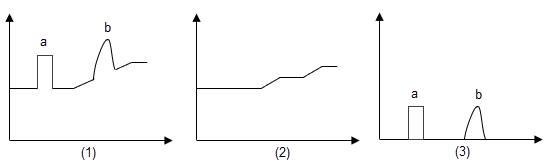
In the illustration above, figure (1) shows a cross-section view of an input DEM with two objects identified (a and b). Figure (2) shows the DEM after the erosion and dilation operations, with objects a and b replaced by the surrounding values. Figure (3) shows output raster with the extracted objects a and b, resulting from by subtracting cross section (2) from (1).
The following explains how the tool calculates the output for the Ridge analysis type.
For each cell, the minimum for its neighborhood is found and assigned to the current cell.
Using the result from step 1, the maximum for each cell's neighborhood is found and assigned to the current cell.
The result from step 2 is subtracted from the input surface raster. The cell values represent the height of the ridges.
Valley analysis
The Valley analysis type corresponds to the black top hat transform function in Rodriguez, et al, 2002. It also performs a series of focal calculations on the input DEM, but the sequence is reversed so that a focal maximum calculation is followed by a focal minimum calculation. Then, the original DEM is subtracted from the result.
The following explains how the tool calculates the output for the Valley analysis type.
For each cell, the maximum for its neighborhood is found and assigned to the current cell.
Using the result from step 1, the minimum for each cell's neighborhood is found and assigned to the current cell.
The input surface raster is subtracted from the result from step 2. The cell values represent the depth of the valleys.
Neighborhood types
The shape of a neighborhood can be a circle or a rectangle. You can also define a custom neighborhood shape by using a kernel file.
Following are descriptions of the neighborhood shapes and how they are defined.
Circle
A circle neighborhood is created by specifying a radius value.
The radius is identified in cell or map units, measured perpendicular to the x- or y-axis. When the radius is specified in map units, additional logic is used to determine which cells are included in the processing neighborhood. First, the exact area of a circle defined by the specified radius value is calculated. Next, the area is calculated for two additional circles: one with the specified radius value rounded down, and one with the specified radius value rounded up. These two areas are compared to the result from the specified radius, and the radius of the area that is closest will be used in the operation.
The default circle neighborhood radius is three cells.
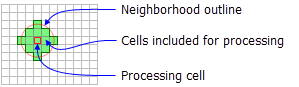
An example illustration of a circle neighborhood follows:
Rectangle
The rectangle neighborhood is specified by providing a width and a height in either cells or map units.
Only the cells with centers that fall within the defined object are processed as part of the rectangle neighborhood.
The default rectangle neighborhood is a square with a height and width of three cells.
The x,y position for the processing cell within the neighborhood, with respect to the upper left corner of the neighborhood, is determined by the following equations:
x = (width of the neighborhood + 1) / 2
y = (height of the neighborhood + 1) / 2
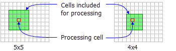
If the input number of cells is even, the x,y coordinates are computed using truncation. For example, in a 5-by-5 cell neighborhood, the x- and y-values are 3,3. In a 4-by-4 neighborhood, the x- and y-values are 2,2.
The following shows two rectangle neighborhoods examples:
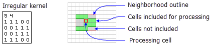
Irregular
Use this option to specify an irregularly shaped neighborhood around the processing cell.
The irregular kernel file specifies the cell positions to be included within the neighborhood.
The x,y position for the processing cell within the neighborhood, with respect to the upper left corner of the neighborhood, is determined by the following equations:
x = (width + 1) / 2
y = (height + 1) / 2
If the input number of cells is even, the x- and y-coordinates are computed using truncation.
The following points apply to a kernel file for an irregular neighborhood:
The irregular kernel file is an ASCII text file that defines the values and shape of an irregular neighborhood. The file can be created with any plain text editor. It must have a
.txtfile extension and no spaces in the file name.The first line specifies the width and height of the neighborhood (the number of cells in the x direction, followed by a space, and the number of cells in the y direction).
The subsequent lines define the value to use for each position in the neighborhood they represent. A space between each value is necessary.
The values define whether a position in the neighborhood will be included in the calculation. Typically, the value 1 is used to identify the positions to include in the calculations for an irregular neighborhood, but any positive or negative value other than 0 can be used. Floating point values can also be used.
To exclude a location in the neighborhood from the calculation, use a value of 0 (not a blank space) at the corresponding location in the kernel file.
The following example shows the contents of an irregular kernel file and the neighborhood it represents:
Reference
Rodriguez, F., E. Maire, P. Courjault-Rade, and J. Darrozes. 2002. "The Black Top Hat function applied to a DEM: A tool to estimate recent incision in a mountainous watershed (Estibere Watershed, Central Pyrenees)." Geophysical Research Letters 29(6): 9.1–9.4.