Esri Income Tiers and Measures of Income Inequality
Esri creates Income Tiers and Measures of Income Inequality data as part of the Updated Demographics dataset for the United States. This topic describes the methodology used to create that data.
Tip:
Esri also provides a copy of this topic as a technical paper: 2026/2031 Esri Income Tiers and Measures of Income Inequality (PDF).
About Esri's Income Tiers and Measures of Income Inequality
Household income survey data is commonly reported as an ordered categorical distribution, along with summary measures of median and average household income. These summary measures provide a description of an area's income profile but give limited information about the shape of the income distribution. The shape, or dispersion, of this data is what can be quantified to define levels or degrees of income inequality.
Fundamentally, income inequality measures the disparity of incomes across households. To better characterize and compare income distributions, Esri has quantified lower, middle, and upper tiers of households by income and provided a full suite of income inequality measures. All metrics are built on EsriUpdated Demographics current and forecast year estimates of households by income.
Income tiers
Esri's approach to income tiers is an adaptation of Nobel Laureate Robert Solow's quintile approach ¹ to defining the middle-class population. Solow, an economist, defines the middle class as the middle 60 percent of earners. This definition has the additional benefit of being symmetric around the median. It follows that the top 20 percent can be considered upper class and the bottom 20 percent lower class. Hence, the size of the middle class can never change, but the range of incomes defining the middle class can. Esri's methodology builds on this country-level definition to classify households into tiers of income for small-area analysis.
Esri's method measures household income distribution. The middle 60 percent is labeled the middle tier of income. Households not identified as middle income are classified into lower-tier and upper-tier categories. Evaluating the tails of the income distribution provides insight into income dispersion in an area (see the Income inequality measures section below). Evaluating changes to the size of the lower- and upper-income tiers over time is an expedient way to understand shifts in the middle-income population. Growth in the middle class will shift households from the lower or upper tiers, or both. When the middle class is in decline, you can begin to answer policy questions such as "Are the rich getting richer?" or "Are the poor getting poorer?" Where local economies foster job growth and government policies support low-income households, households are expected to move up the income ladder over time. In areas experiencing gentrification, however, income shifts may reduce the size of the low- and middle-income tiers while expanding the upper income tier.
Esri's methods establish Census division-level quintile limits as criteria to define the range of household incomes considered middle-income tier. Employing division-level limits (versus U.S. limits) accounts for geographic variability in the cost of living. Therefore, households earning the same income in the more relatively expensive Pacific division versus the East South-Central division are not necessarily classified using the same thresholds. By way of Esri's household income estimates, these division-level criteria are updated annually. At the division level of geography and above, the sizes of the lower, middle, and highest tiers do not change over time. This data captures shifts in the size of each income tier for underlying smaller areas.
Esri has developed a methodology to estimate middle-tier households at any level of geography and is amenable to trending over time. Households by income tiers are first established at the Census block group level using Pareto interpolation to distribute households into each grouping. Estimates of income tiers for other geographic summary areas are aggregated from this foundational level. An important consideration is that, at the national level, middle-tier households may represent slightly more or less than 60 percent of the total. Estimates for user-defined polygons are produced using established geometric retrieval techniques. The criteria for assigning households to the lower, middle, and upper tiers for the 2026 estimates are presented in the table below.
| Division | Lower tier | Middle tier | Upper tier |
|---|---|---|---|
| New England | <$40,773 | $40,773 - $205,972 | >$205,972 |
| Middle Atlantic | <$36,220 | $36,220 - $188,972 | >$188,972 |
| East North Central | <$34,425 | $34,425 - $156,429 | >$156,429 |
| West North Central | <$36,105 | $36,105 - $155,506 | >$155,506 |
| South Atlantic | <$35,934 | $35,934 - $169,289 | >$169,289 |
| East South Central | <$28,694 | $28,694 - $139,741 | >$139,741 |
| West South Central | <$32,568 | $32,568 - $160,437 | >$160,437 |
| Mountain | <$39,709 | $39,709 - $171,930 | >$171,930 |
| Pacific | <$42,421 | $42,421 - $209,613 | >$209,613 |
The following chart shows an example of two sample areas X and Y with bottom- and top-heavy income distributions, respectively. Both show very different distributions across income tiers. With these extreme examples, it is obvious that area X has a dominant upper tier and area Y has a dominant middle tier.
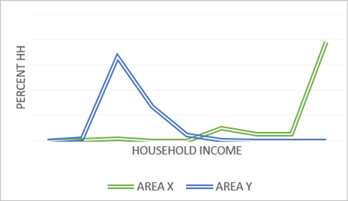
The table below shows the percent of households by income tier for areas X and Y:
| Tier | Area X (% Households) | Area Y (% Households) |
|---|---|---|
| Lower | 1.0 | 25.1 |
| Middle | 15.1 | 74.9 |
| Upper | 83.9 | 0.0 |
In more concentrated income distributions, one income tier is dominant. When the income range in an area is broad or less concentrated in and around one income interval, quantifying the spread of incomes across tiers is more valuable for comparative analyses. The following two chart examples show income distributions and tiers for the largest counties in the Northern Virginia area.
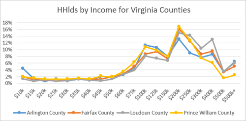
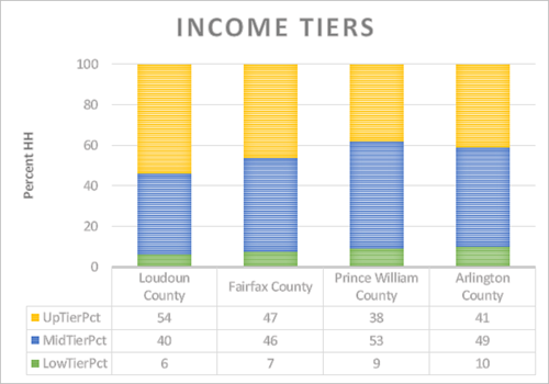
Summarizing the households by income into three tiers puts the information in a more interpretable and comparative format. Income distributions for these four counties exhibit the same general pattern, with higher income tiers representing the largest share in three of the four counties. The income tiers not only reveal sociodemographic groupings but are also comparative between areas. Prince William County has the largest portion of middle-tier households while Loudoun County, with relatively newer development, consists of predominantly upper-tier households. Arlington County and Fairfax County show a relatively better balance between middle- and upper-tier households. Studying income inequality provides further insight, allowing the analyst to understand the dispersion of incomes across tiers by quantifying the income divide.
Income inequality measures
Evaluating the tails of an area's income distribution provides insight into the unevenness or spread of household incomes—in other words, income inequality. Inequality measures are most often developed to study relative differences across countries. Esri applies the same principles to provide a full suite of inequality–focused metrics geographically available from the neighborhood level and broader to complement an analysis. All measures are designed to compare inequality across different markets regardless of size; they are scale independent. Key measures include the following:
Gini Index
Interdecile ratios
90-10
50-90
50-10
Share ratios
80-20
90-40 (Palma ratio)
Gini Index
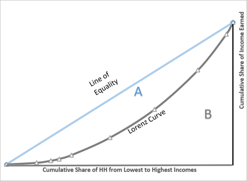
The Gini Index is a measure of income dispersion. It is independent of income levels. Specifically, the calculation measures deviation from a hypothetical 45-degree line representing perfect equality where every household in an area earns the same income. In theory, the calculation is developed using the Lorenz curve shown below, which plots the cumulative share of income against the cumulative share of households.
The computation of the Gini Index evaluates the area between the diagonal line representing equality and the Lorenz curve capturing the aggregate income distribution for the area being evaluated. Referring to the first chart below, the Gini Index is the ratio of area A divided by the sum of areas A and B. The range of the Gini Index is 0 to 100, where 0 is perfect equality and 100 is complete inequality. Varying levels of the Gini Index are demonstrated graphically on the Lorenz curve in the second chart below. The third chart shows the Lorenz curve and Gini Indices for the four Northern Virginia counties in the tables discussed previously in this topic.
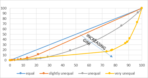
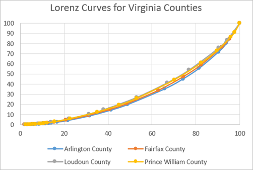
A Gini Index is one of the most frequently used measures to track income inequality; however, it does not indicate which part of the income distribution contributes most to income inequality. Two areas can have the same Gini Index but differing income distributions. In the example of two areas X and Y, both have a Gini Index of ±10, but the underlying distributions are very different. The Northern Virginia counties show some Gini Index variation, with Loudoun County showing the lowest inequality with a Gini Index of 36.9 and Prince William County and Fairfax County marginally more unequal at 38.3 and 38.9; Arlington County shows higher inequality, with an index of 43. These patterns are also visible in the Lorenz curves for these counties. What we learn is that areas with the most affluent populations are not necessarily the most unequal.
The Gini Index measures deviation from equality in the aggregate; it does not capture differences in the shape of the income distribution. As a stand-alone statistic, it has limited use; however, it is a stable measure that is amenable to time series analysis.
Interdecile ratios
Interdecile ratios highlight income inequalities of a distribution. These measures quantify the spread of incomes across households in any area and are derived from income limits by percentile. Esri provides three common ratios:
P90-10 ratio—Compares income earned by households at the 90th percentile to the income earned by households at the 10th percentile. In other words, it compares the top 10 percent to the bottom 10 percent of the distribution.
P90-50 ratio—Compares income earned by households at the 90th percentile to the income earned by households at the 50th percentile. In other words, it compares the top 10 percent to the median of the distribution.
P50-10 ratio—Compares income earned by households at the 50th percentile to income earned by households at the 10th percentile. In other words, it compares the median to the bottom 10 percent of the distribution.
The P90-10 ratio quantifies an area's equality gap, but it provides little information about the middle section of the income distribution. The P90-50 and P50-10 ratios provide more information; the P90-50 ratio summarizes inequality above the median, while the P50-10 ratio summarizes inequality below the median. The product of the P90-50 and P50-10 ratios is the P90-10 ratio.
At the foundation of this method is the computation of percentile limits for the underlying income distribution. Esri's measures rely on a categorical distribution: households by income intervals. Like the median estimation methods, a percentile limit is calculated from the income intervals of the distribution using Pareto interpolation unless the limit falls in the lowest (<$15,000) or highest (>$500,000) interval. For the lowest interval, linear interpolation is used.
The below chart demonstrates the relationship between percentile limits and households. It displays the estimated U.S. quintile limits (the 20th, 40th, 60th, and 80th percentile limits). These dollar values divide total U.S. households into equal bins representing 20 percent of the population.
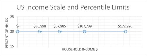
The shape of the income distribution determines the scale; the spread of quintiles is demonstrated in the following two quintile charts for area X and area Y. Regardless of the dollar value of the quintile limits, the same number of households are in each of the five quintile groups. The concentration of household incomes in area Y is illustrated by quintile limits falling within a very small range.
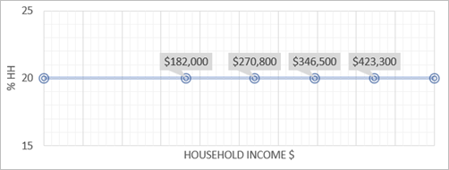
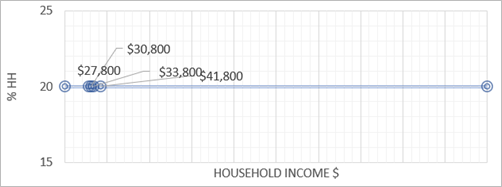
Though both areas have similar Gini Index values, interdecile ratios (as shown in the table below) shed more light on the shape of the distribution. Interdecile ratios capture the relationship between percentile limits into one comparative metric. The P90-10 ratio for area X exceeds that of area Y by more than a factor of 2.5, indicating that there is a wider range of household incomes in area X than in area Y. Area X is more unequal than area Y, as indicated by the P90-10 ratio. Breaking this down into the P90-50 and P50-10 ratios confirms that the difference in inequality for these two areas is driven by inequality below the median. This shows that area X has a larger gap or spread between the incomes of households earning the median compared to the households earning at the 10th percentile of the distribution. Inequality above the median is the same between the two.
| Measure | Area X | Area Y |
|---|---|---|
| P90-10 ratio | 4.8 | 1.8 |
| P90-50 ratio | 1.5 | 1.5 |
| P50-10 ratio | 3.2 | 1.2 |
Revisiting the Northern Virginia counties example, the P90-10 ratio offers a more interpretable metric for assessing inequality. Consistent with the Gini Index findings, Loudoun County emerges as the least unequal by this measure. This outcome reflects the relative concentration of income in the upper tier, which narrows the gap between households at the 90th percentile and those at the 10th percentile. The concentration in income in the upper tier is reflected in the lowest P90-50 ratio—meaning that inequality above the median is low. Interdecile ratios show that each of these counties exhibit a considerable difference in inequality above and below the median, as indicated by the P90-50 ratios that are approximately half of the P50-10 ratios.
| Measure | Loudon County | Fairfax County | Prince William County | Arlington County |
|---|---|---|---|---|
| P90-10 ratio | 7.3 | 8.1 | 7.6 | 11.1 |
| P90-50 ratio | 2.1 | 2.3 | 2.1 | 2.8 |
| P50-10 ratio | 3.6 | 3.5 | 3.6 | 4.0 |
Share ratios
Interdecile ratios are positional measures while share ratios also reflect aggregate income earned by the highest earners relative to the lowest earners. Two share measures are developed by Esri:
S80-20 share ratio—This measure compares the total income of households earning at or above the 80th percentile to the total income of households earning at or below the 20th percentile. In other words, the ratio of the income earned by the upper tier to the income earned by the lower tier, effectively providing a direct comparison between households outside the middle tier.
S90-40 share ratio—This measure compares the total income of households earning at or above the 90th percentile to the total income of households earning at or below the 40th percentile. Commonly referred to as the Palma ratio ², proposed by Alex Cobham and Andy Sumner based on the work of Gabriel Palma, whose research concluded that 50 percent of households (those earning between the 40th and 90th percentiles) earned 50 percent of the national income, across all countries in the study. The stability of this middle income share over time combined with the relative instability of the lowest 40 percent and uppermost 10 percent of earners is the foundation of this inequality measure.
To derive these measures, Esri applies Pareto interpolation techniques to distribute aggregate income using subinterval midpoints to above and below the defined limit of income.
Share ratios can describe a much different picture of income dispersion. Whereas interdecile ratios are strictly positional, share ratios accommodate both aggregate (embedded in the Gini Index calculation) and positional criteria. The S80-20 share ratio is a symmetric measure that exaggerates income inequality compared to the S90-40 share ratio. This is demonstrated by the share ratios for area X, which has a top-heavy distribution and reflects higher values in the S80-20 share than the S90-40 share. The S80-20 share ratio widens the gap between areas X and Y, while the difference in the S90-40 share ratio is significantly muted, as shown in the below table:
| Measure | Area X | Area Y |
|---|---|---|
| S80-20 ratio | 12.6 | 1.7 |
| S90-40 ratio | 3.3 | 0.6 |
Again referencing the Northern Virginia counties, the S80-20 and S90-40 share ratios describe a different picture of inequality, ranking Loudoun County as the most unequal. Share ratios are much more sensitive to differences in the uppermost income category, as is the case in these two counties. This is best explained by the change to a county's aggregate income when one household moves into an area. The presence of one additional household earning $200,000 adds 10 times the income when compared to the addition of a household earning $20,000. This multiple is built directly into the share ratios.
| Measure | Loudon County | Fairfax County | Prince William County | Arlington County |
|---|---|---|---|---|
| S80-20 ratio | 7.1 | 8.3 | 7.2 | 10.7 |
| S90-40 ratio | 1.5 | 1.8 | 1.5 | 2.2 |
Limitations of the data
Esri follows the U.S. Census Bureau's practice of top-coding median household income. When the median falls in the upper interval, it is reported as $500,001 because households in the upper interval are top coded to $500,000. This will add a negative bias to all income inequality measures computed for areas with any households earning $500,000 or more. To reduce this bias in the computation of inequality statistics, Esri's methods apply Pareto interpolation to households in this income group, assuming an upper limit of $500,000. Error is also introduced because Esri's methods must rely on ordinal data (ordered and grouped households by income).
To understand bias in the data, it is useful to examine income inequality measures in reported national survey data. Below are U.S. level income inequality statistics compared against American Community Survey (ACS) and Current Population Survey (CPS) figures. The American Community Survey (ACS) reports only the Gini Index as its measure of income inequality. Other metrics are calculated internally by Esri using a nine-interval income distribution comparable to Esri's own distribution model. Esri employs ACS estimates as the foundation for its household income estimates, making the ACS the most appropriate source for comparison with Esri measures. Because ACS estimates serve as the base, both ACS and Esri income inequality measures are subject to the same top-coding limitations.
Income inequality measures reported directly from the CPS are also presented here. ACS and CPS survey methodology, including the household income definition, are significantly different and will impact comparability of these sources. It is worth reviewing CPS income inequality metrics because they are not subject to the same top-coding restrictions. Note that all Esri and internally calculated ACS ratios run lower than the CPS, further proving the negative bias that is assumed in Esri computed metrics (the exception is of course the P50-10 ratio, which is not impacted by top-coding at the national level). Caution must therefore be used when comparing metrics across sources.
| Measure | 2024 ACS ³ | 2024 CPS | Esri 2026 U.S. |
|---|---|---|---|
| Gini Index | 46.9 4 | 48.8 | 46.7 |
| P90-10 ratio | 12.8 | 12.6 | 13.0 |
| P90-50 ratio | 2.9 | 3.0 | 2.8 |
| P50-10 ratio | 4.5 | 4.2 | 4.6 |
| S80-20 ratio | 10.1 | 14.4 | 10.6 |
| S90-40 ratio | 2.1 | n/a 5 | 2.1 |
All survey data is subject to sampling and non-sampling errors, and derived metrics have inherent limitations even with the benefit of detailed income data. Esri income metrics are subject to top coding and categorical data bias, but with an understanding of these assumptions, when used together, the inequality metrics provide users with a more holistic portrait of income disparities.
References
See the following references for additional information:
Estache, Antonio and Danny Leipziger. eds. 2009. "Stuck in the Middle: Is Fiscal Policy Failing the Middle Class?" Washington, DC: Brookings Institution Press. ISBN: 978-0-815-70284-9
Cobham, Alex and Sumner, Andy, September 16, 2013. "Is It All About the Tails? The Palma Measure of Income Inequality" Center for Global Development Working Paper No. 343, Available at SSRN:
https://ssrn.com/abstract=2366974orhttp://dx.doi.org/10.2139/ssrn.2366974.All ratio calculations follow Esri's practice of disaggregating households and their aggregate income into percentile bins at the block group level. Ratio computation is based on aggregated BG data.
Esri internal calculation based on ACS one-year collapsed sixteen-interval distribution. The reported ACS 2023 Gini Index is 0.483.
Not published by CPS.