Estimating cross-covariance models for cokriging
 Available with Geostatistical Analyst license.
When you have multiple datasets and you want to use cokriging, you need to develop models for cross-covariance. Because you have multiple datasets, you keep track of the variables with subscripts, with Zk(s j) indicating a random variable for the kth data type at location s i. The cross-covariance function between the kth data type and the mth data type is then defined to be
\(C \space _{ \textit{km} } \space ( \textbf{s} _{i} , \textbf{s} _{j} ) \space = \space cov(Z _{k} ( \textbf{s} _{i} ), \space Z _{m} ( \textbf{s} _{j} ))\)
Here is a subtle and often confusing fact: C km (s i , s j) can be asymmetric: C km (s i , s j) ≠ C mk (s i , s j) (notice the switch in the subscripts). To see why, look at the following example. Suppose you have data arranged in one dimension, along a line, such as the following:

The variables for type 1 and 2 are regularly spaced along the line, with the thick red line indicating highest cross-covariance, the green line less cross-covariance, and the thin blue line the least cross-covariance, with no line indicating 0 cross-covariance. This figure shows that Z1(s i) and Z2(s j) have the highest cross-covariance when s i = s j, and the cross-covariance decreases as s i and s j get farther apart. In this example, C km (s i , s j ) = C mk (s i , s j ). However, the cross-covariance can be "shifted":
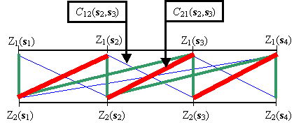
Notice that C12(s 2, s 3) now has the minimum cross-covariance (thin blue line) while C21(s 2, s 3) has the maximum cross-covariance (thick red line), so here Ckm (s i , s j) ≠ C mk (s i , s j). Relative to Z1, the cross-covariances of Z2 have been shifted -1 unit. In two dimensions, Geostatistical Analyst will estimate any shift in the cross-covariance between the two datasets if you click the shift parameters.
The empirical cross-covariances are computed as follows:
Average [ (z1(si) -  1) (z2(sj) - 2)]
where Zk(s i) is the measured value for the kth data set at location s i , k is the mean for the kth dataset, and the average is taken for all s i and s j separated by a certain distance and angle. As for the semivariograms, Geostatistical Analyst shows both the empirical and fitted models for cross-covariance.
Choosing different cross-covariance models, using compound cross-covariance models, and choosing anisotropy will all cause the theoretical model to change. You can make a preliminary choice of model by seeing how well it fits the empirical values. Changing the lag size and the number of lags and adding shifts will change the empirical cross-covariance surface, which will cause a corresponding change in the theoretical model. Geostatistical Analyst computes default values, but you should feel free to try different values and use validation and cross-validation to choose the best model.