How Radial Roughness works
 Available with the Spatial Analyst license.
The Radial Roughness tool calculates a short-range omnidirectional roughness value for each cell of an input surface raster, using the radial roughness index approach (Trevisani, et al, 2023). The output roughness value is a measure of the height differences between the current cell and its neighboring cells, with the following characteristics:
The output roughness value is independent of the local slope.
During the calculation, the distance between cell centers is adjusted along the ordinal directions using bilinear interpolation.
The lowest possible value on the output raster is 0, which represents a smooth area. A more rugged area will have a higher value.
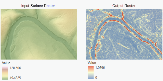
The following are some application examples using the output roughness raster:
Identifying rough and smooth terrains on a digital elevation model (DEM) using the roughness values
Using it as a layer in land use suitability modeling
Using it as a cost raster in cost distance analysis to identify a smooth walking path in a recreation area
Radial roughness algorithm
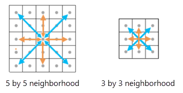
For any given output cell, the tool calculates a final roughness value from 12 directional differences from two different neighborhood sizes. To do this, the tool goes through the following steps:
For a 5-by-5 cell neighborhood, calculate the second-order difference values in eight directions.
For a 3-by-3 cell neighborhood, calculate the second-order difference values in four directions.
Calculate the final roughness value by averaging the 12 values resulting from the previous two steps.
The following illustrates which input values contribute to the calculation of the differences in the cardinal (orange) and ordinal (light blue) directions around the processing cell. The graphic on the left represents the 5-by-5 cell neighborhood, and the graphic on the right represents the 3-by-3 cell neighborhood.
Compute second-order differences in the 5-by-5 neighborhood
The difference in values between two adjacent cells is a first-order difference. A second-order difference is the difference in the differences in the cell values between two adjacent pairs of cells. This tool uses a second-order difference approach when computing the cell value differences. It allows the effect of the local slope to be removed in the final output roughness values. The following sections present the formulas used by the tool to compute the differences along the eight directions for a 5-by-5 neighborhood.
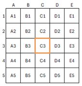
The specific cells used in the formulas are identified by their column and row as follows:
Second-order differences in the cardinal directions
The four cardinal directions are East, South, West, and North. Using the cells in the East direction of the neighborhood as an example, the absolute value of the second-order difference for that direction is calculated as follows:
\(D_1 = | (Z_{D3} - Z_{E3}) - (Z_{C3} - Z_{D3}) | = | 2 * Z_{D3} - Z_{C3} - Z_{E3} |\)
Where Z is the cell value for a given cell in the neighborhood.
Similarly, for the South direction, the formula is as follows:
\(D_2 = | 2 * Z_{C4} - Z_{C3} - Z_{C5} |\)
For the West direction:
\(D_3 = | 2 * Z_{B3} - Z_{C3} - Z_{A3} |\)
For the North direction:
\(D_4 = | 2 * Z_{C2} - Z_{C3} - Z_{C1} |\)
Second-order differences in the ordinal directions
The four ordinal directions are Northeast, Southeast, Southwest, and Northwest. Because the distance between cell centers is greater than one cell along the ordinal directions, bilinear interpolation is used to get the cell values along these directions with the distance of 1 cell.
Using the Northeast direction as an example, with the bilinear interpolation weights considered, the following is the formula for calculating the second-order difference in that direction (Trevisani, et al, 2023):
\(D_5 = | -0.5 * Z_{C3} - 0.5 * Z_{E1} - 0.2071 * Z_{C2} - 0.2071 * Z_{D1} - 0.2071 * Z_{D3} - 0.2071 * Z_{E2} + 1.8284 * Z_{D2} |\)
Where Z represents the cell value for a given cell in the neighborhood.
Similarly, for the Southeast direction, the formula is as follows:
\(D_6 = | -0.5 * Z_{C3} - 0.5 * Z_{E5} - 0.2071 * Z_{D3} - 0.2071 * Z_{E4} - 0.2071 * Z_{C4} - 0.2071 * Z_{D5} + 1.8284 * Z_{D4} |\)
For the Southwest direction:
\(D_7 = | -0.5 * Z_{C3} - 0.5 * Z_{A5} - 0.2071 * Z_{B3} - 0.2071 * Z_{A4} - 0.2071 * Z_{C4} - 0.2071 * Z_{B5} + 1.8284 * Z_{B4} |\)
For the Northwest direction:
\(D_8 = | -0.5 * Z_{C3} - 0.5 * Z_{A1} - 0.2071 * Z_{C2} - 0.2071 * Z_{B1} - 0.2071 * Z_{B3} - 0.2071 * Z_{A2} + 1.8284 * Z_{B2} |\)
Compute second-order differences in the 3-by-3 neighborhood
In the 3-by-3 neighborhood, the four directions along which the differences are computed are East-West, North-South, Northeast-Southwest and Northwest-Southeast. The following are the formulas for those.
For the East-West direction:
\(D_9 = | 2 * Z_{C3} - Z_{B3} – Z_{D3} |\)
For the North-South direction:
\(D_{10} = | 2 * Z_{C3} - Z_{C2} – Z_{C4} |\)
For the Northeast-Southwest direction:
\(D_{11} = | -0.5 * Z_{B4} - 0.5 * Z_{D2} - 0.2071 * Z_{B3} - 0.2071 * Z_{C2} - 0.2071 * Z_{C4} - 0.2071 * Z_{D3} + 1.8284 * Z_{C3} |\)
For the Northwest-Southeast direction:
\(D_{12} = | -0.5 * Z_{D4} - 0.5 * Z_{B2} - 0.2071 * Z_{C4} - 0.2071 * Z_{B3} - 0.2071 * Z_{D3} - 0.2071 * Z_{C2} + 1.8284 * Z_{C3} |\)
Additional resources
See the following for more information:
- Trevisani, S., Teza, G., and Guth, P.L., 2023. "Hacking the topographic ruggedness index". Geomorphology, 439, Article: 108838. https://doi.org/10.1016/j.geomorph.2023.108838