Summarize Attributes (Real-time) (Beta)
 Available in real-time analytics.
The Summarize Attributes tool  summarizes field values to generate a summary table. The resulting output table displays the count of summarized features and any additional specified statistics.
Workflow diagram
Examples
Managing assets and sensor data can be challenging with high-frequency, real-time observations. Although individual data points show what an asset or sensor is doing at a specific moment, analyzing rolling subsets of incoming data can provide a broader view of conditions and trends over time.
The following are example use cases for the tool:
Adding values for the Mean, Min, Max, and Standard Deviation options for the last 10 vehicle speed observations by track ID can help identify erratic driving or traffic slowdowns.
Adding values for the Mean option temperature, vibration, and pressure options over the last five minutes by track ID can help detect hazardous conditions.
The Mean option value for processing time, Max option value for wait time, and total facility gate event count across the last 100 events can help power a live operations dashboard.
Adding values for the Min, Max, and Mean air quality index options over the last 10 minutes for an environmental sensor can provide an overall view of air health.
Usage notes
Note the following when working with the tool:
Inputs can be tabular layers or layers with geometry (points, lines, or areas) and must be time-enabled. Features without a time value are not processed.
This tool provides the following scope choices for calculations with the State Mode parameter (choose only one mode at a time):
The Track-based mode maintains rolling summary statistics separately for each track ID, using the
Track IDfield defined in the input schema.The Summary set mode maintains one rolling summary across all incoming features, without separating observations by track ID.
To calculate statistics from previous observations, the tool temporarily retains recent observations in a state store. The Calculation Mode parameter determines how much data is retained and used in each rolling calculation (choose only one mode at a time):
The History Depth mode retains and calculates statistics from a specified number of observations, including the current observation.
The Time Window mode retains and calculates statistics from observations within a specified time window, using each observation's event start time.
When you choose the Track-based mode, the input must include a field tagged as
Track ID. The tool uses this field to maintain a separate rolling summary for each track.This tool is a tabular analysis tool, not a spatial analysis tool. You can use this tool with spatial data. However, the result is tabular. For more information, refer to the Output table section.
The output table of this tool always includes a count of the number of features that the tool has summarized. If you also choose Count for a summary field, the output includes an additional field-specific count.
Use the Summary fields parameter to calculate additional statistics. The summary fields statistics available depend on the field type you are summarizing.
A string attribute field can use the Any, Count, and Count (distinct) statistics.
A numeric attribute field can use the Any, Count, Count (distinct), Sum, Sum of Squares, Min, Max, Mean, Range, Variance, and Standard Deviation statistics.
A date attribute field can use the Any, Count, Min, Max, and Range statistics.
How the tool works
The Summarize Attributes tool first reviews the Calculation Mode parameter and stores incoming real-time data in a state store according to the setting chosen.
In the History Depth mode, the tool retains up to the configured number of recent observations and recalculates summary statistics as each feature is processed. Each calculation includes the current observation and as many previous observations as needed to reach the configured depth. If fewer observations are available for a track or summary set, the calculation uses those available.
For the Time Window mode, the tool runs calculations immediately with any data available in the state store.
The tool then runs calculations based on the State Mode parameter.
For the Track-based mode, the tool runs calculations on subsets of data organized by the input
Track IDfield.For the Summary set mode, the tool runs calculations on the entire dataset in the state store, as if the entire dataset were under a single
Track IDfield.
The following sections describe equations, calculations, parameters, and the output table.
Equations
Variance is calculated using the following equation:
\(s^2 = \left( \frac{\sum_{i=1}^{N} x_i^2 - N\bar{x}^2}{N-1} \right)\)
Where:
\(s^2\) is the variance.
\(N\) is the number of observations.
\(x_i\) is the value of each observation.
\(\bar{x}\) is the mean of the observations.
Standard deviation is calculated as the square root of the variance.
Calculations
The Summarize Attributes tool calculates rolling summary statistics from observations stored in the tool state store. For example, a logistics team can use stop-completion events from delivery vehicles to summarize how many packages were delivered at recent stops, such as businesses, apartment buildings, or pickup locations.
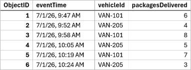
When you set State Mode to Track-based, Calculation Mode to History Depth, and History Depth to 2, the tool summarizes the two most recent stops for each vehicle. This can help answer questions such as, "How many packages did each vehicle deliver during its two most recent stops?"
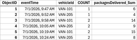
In table 2, each row shows the sum of packages delivered for the two most recent stops of the vehicle in that event. The tool calculates these values by referencing the packages delivered at each stop in table 1:
At 7/1/2026 9:47 a.m., only one stop has occurred for VAN-101, so
COUNTremains 1 andpackagesDelivered_Sumis 6.At 7/1/2026 9:52 a.m., only one stop has occurred for VAN-205, so
COUNTremains 1 andpackagesDelivered_Sumis 4.At 7/1/2026 9:58 a.m., using VAN-101's two most recent stops at 9:47 a.m. and 9:58 a.m.,
COUNTremains 2 andpackagesDelivered_Sumis 6 + 8 = 14.At 7/1/2026 10:05 a.m., using VAN-205's two most recent stops at 9:52 a.m. and 10:05 a.m.,
COUNTremains 2 andpackagesDelivered_Sumis 4 + 5 = 9.At 7/1/2026 10:19 a.m., using VAN-101's two most recent stops at 9:58 a.m. and 10:19 a.m.,
COUNTremains 2 andpackagesDelivered_Sumis 8 + 7 = 15.At 7/1/2026 10:24 a.m., using VAN-205's two most recent stops at 10:05 a.m. and 10:24 a.m.,
COUNTremains 2 andpackagesDelivered_Sumis 5 + 3 = 8.
When you set State Mode to Summary set, Calculation Mode to Time Window, and Time Window to 30 minutes, the tool summarizes all stops that occurred within the rolling time window. This can help answer questions such as, "How many stops occurred and how many packages were delivered by the fleet during the last 30 minutes?"
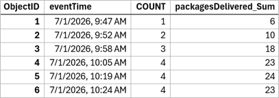
In table 3, each row shows the count and sum of packages delivered by the entire fleet within the rolling 30-minute window. The tool calculates these values by referencing the event times and packages delivered at each stop in table 1:
At 7/1/2026 9:47 a.m., only the 9:47 a.m. event has occurred, so
COUNTremains 1 andpackagesDelivered_Sumis 6.At 7/1/2026 9:52 a.m., the 9:47 a.m. and 9:52 a.m. events fall within the last 30 minutes, so
COUNTremains 2 andpackagesDelivered_Sumis 6 + 4 = 10.At 7/1/2026 9:58 a.m., the 9:47 a.m., 9:52 a.m., and 9:58 a.m. events fall within the last 30 minutes, so
COUNTremains 3 andpackagesDelivered_Sumis 6 + 4 + 8 = 18.At 7/1/2026 10:05 a.m., the 9:47 a.m., 9:52 a.m., 9:58 a.m., and 10:05 a.m. events fall within the last 30 minutes, so
COUNTremains 4 andpackagesDelivered_Sumis 6 + 4 + 8 + 5 = 23.At 7/1/2026 10:19 a.m., the 9:47 a.m. event does not fall within the 30-minute window and is dropped, but the 9:52 a.m., 9:58 a.m., 10:05 a.m., and 10:19 a.m. events fall within the last 30 minutes, so
COUNTremains 4 andpackagesDelivered_Sumis 4 + 8 + 5 + 7 = 24.At 7/1/2026 10:24 a.m., the 9:47 a.m. and 9:52 a.m. events do not fall within the 30-minute window and are dropped, but the 9:58 a.m., 10:05 a.m., 10:19 a.m., and 10:24 a.m. events fall within the last 30-minute window, so
COUNTremains 4 andpackagesDelivered_Sumis 8 + 5 + 7 + 3 = 23.
Parameters
The following table describes the parameters for the tool:
|
Parameters |
Explanation |
Data type |
|---|---|---|
|
Input layer |
The input with features that will be summarized. |
Features |
|
State Mode |
Choose how the incoming features are used for each rolling summary calculation. Choose one of the following:
|
String |
|
Calculation Mode |
Choose how much data to retain in the state store and use for your rolling calculations. Choose one of the following:
Only one calculation mode can be selected. |
String |
|
History Depth |
If you choose the History Depth mode for the Calculation Mode parameter, this parameter specifies the maximum number of recent observations used in each calculation, including the current observation. For example, a value of five uses the current observation and up to four previous observations. The tool produces an output for each processed feature. If a track or summary set contains fewer observations than the configured History Depth value, the calculation uses all observations in that track or summary set. The default is 5. |
Integer |
|
Time Window |
If you choose the Time Window mode for the Calculation Mode parameter, specify the rolling duration of time to cache observations in the state store. The start time is used to determine which observations to include. In Time Window mode, this tool begins calculating as soon as data is available in the state store. The tool displays a warning when the Time Window mode exceeds 24 hours, because longer windows can affect performance. The default is 5 minutes. Options for units are seconds, minutes, or hours. |
String |
|
Summary fields (optional) |
The statistics calculated for the specified fields. Available statistics vary based on whether the field is a string, numeric, or date field. The supported statistics types are as follows:
|
String |
Output table
The output table includes summarized attributes that you specify with the Summary fields (optional) parameter. It also includes event time fields, which help identify results and support downstream joins, and the Track ID field when you choose the Track-based mode. Each output row includes a COUNT field showing the number of features in that rolling summary. This is separate from the Count statistic, which counts nonnull values in a specified summary field. To reduce state store size, the output table does not preserve geometry and other input fields. You can rejoin these fields using the Join Features tool.
If you use a spatiotemporal feature layer as an output type, the tool creates both a spatiotemporal feature layer and a map image layer. If you use an ArcGIS Online hosted feature layer as an output type, the output table is a Table (hosted).