Reconstruct Tracks (GeoAnalytics Server Tools)

Summary

Creates line or polygon tracks from time-enabled input data.

Legacy:

The ArcGIS GeoAnalytics Server extension is being deprecated in ArcGIS Enterprise. The final release of GeoAnalytics Server was included with ArcGIS Enterprise 11.3. This geoprocessing tool is available through ArcGIS Enterprise 11.3 and earlier versions.

Illustration

Usage

• Reconstruct Tracks is run on point or polygon features. The input layer must be time enabled with features that represent an instant in time.

• You can specify one or more fields to identify tracks. Tracks are represented by the unique combination of one or more track fields. For example, if the fields flightID and Destination are used as track identifiers, the features ID007, Solden and ID007, Tokyo would be in two separate tracks, since they have different Destination field values.

• Features that have a buffer applied will result in polygonal tracks. Input point features that do not have a buffer applied will result in polyline tracks.

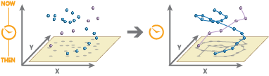
• Input features will consist of time-enabled features that represent an instant in time. Results are line or area features that represent an interval in time. The start and end of the interval are determined by the time at the first and last features in a track.

  

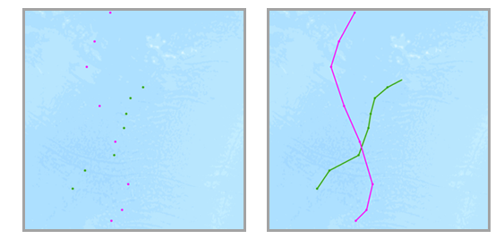
  The input features with two distinct tracks (green and red) that have time type instant (left) and the resulting tracks (right) or time type interval are shown.

• For linear results, only tracks that contain more than one point will be returned. If you apply a buffer, all features will be returned.

• You can optionally apply a buffer to your input features. When you apply a buffer, the resulting tracks will be polygon features.

  

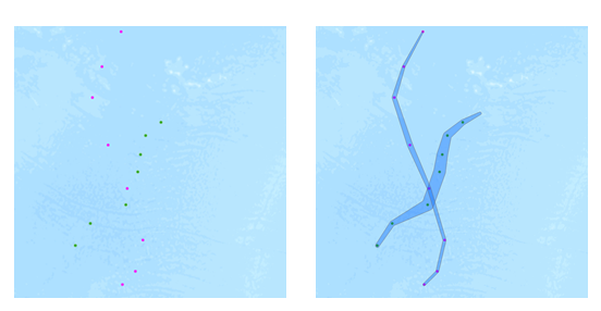
  Input points with a buffer applied are reconstructed into tracks.

• When buffering input features, each input feature is buffered. Then a convex hull is generated to create a polygon track.

  

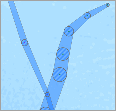
  An example of input points (green), an intermediate buffer for visualization (blue hatching), and the resulting polygonal track (blue) are shown.

• Fields used in the buffer expression must be numeric and will be applied using the units of the input's spatial reference. See Buffer expression examples for ArcGIS Enterprise 10.5 and 10.5.1 or Buffer expression examples for ArcGIS Enterprise 10.6 and later for more information. In ArcGIS Enterprise 10.6.1 or later, you can use track-aware equations.

• By default, only the count of points or polygons in a track will be calculated. Additional statistics can be calculated by specifying the Summary Fields parameter value.

• By default, tracks are created using a geodesic method. The method is applied to the following two components of the analysis:

  • Tracks crossing the international date line—When using the geodesic method, input layers that cross the international date line will have tracks that correctly cross the international date line. This is the default. Your input layer or processing spatial reference must be set to a spatial reference that supports wrapping around the international date line, for example, a global projection such as World Cylindrical Equal Area.

  • Buffers—Input features can optionally be buffered. To learn more about when to apply a geodesic or planar buffer, see Create buffers.

• You can split tracks in the following ways:

  • Time Split—Based on a time between inputs. Applying a time split breaks up any track when input data is farther apart than the specified time. For example, if you have five features with the same track identifier and the times of [01:00, 02:00, 03:30, 06:00, 06:30] and set a time split of 2 hours, any features that are measured more than 2 hours apart will be split. In this example, the result would be a track with [01:00, 02:00, 03:30] and [06:00, 06:30], because the difference between 03:30 and 6:00 is greater than 2 hours.

  • Time Boundary Split—Based on defined time intervals. Applying a time boundary split segments tracks at a defined interval. For example, if you set the time boundary to 1 day, starting at 9:00 a.m. on January 1, 1990, each track will be truncated at 9:00 a.m. every day. This split accelerates computing time, as it creates smaller tracks for analysis. If splitting by a recurring time boundary makes sense for your analysis, it is recommended for big data processing.

  • Distance Split—Based on a distance between inputs. Applying a distance split breaks up any track when input data is farther apart than the specified distance. For example, if you set a distance split of 5 kilometers, sequential features greater than 5 kilometers apart will be part of a different track.

  • Split Expression—Based on an Arcade expression. Applying a split expression splits tracks based on values, geometry or time values. For example, you can split tracks when a field value is more than double the previous value in a track. To do this, using an example field named WindSpeed, you can use the following expression: var speed = TrackFieldWindow("WindSpeed", -1, 1); 2* speed[0] < speed[1]. Tracks will split when the previous value (speed[0]) is less than two times the current value.

• You can apply none, one, two, three, or four split options at the same time. All of the examples below use a gap split. The results, assuming you apply a time split of six hours, a time boundary of one day, and distance split of 16 kilometers, are as follows:

  

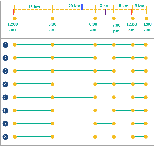
  Five examples of input points (yellow) with varying time and distance splits are shown.

  Split option	Description
  Six input points with a time and location	Input points with the same identifier. The distance between the points is marked on top of the dotted line, and the time of each point measurement is marked below the points. There are four splits on the timeline. The red splits represent the time boundary split of one day starting at 12:00 a.m. The blue split represents the distance split when the distance between two points is greater than 16 kilometers. The purple split represents the time split when the temporal distance between two sequential points is more than six hours.
  	Example with no time split and no distance split.
  	Example with a time split of six hours. Any features more than two hours apart are split into separate tracks.
  	Example with a time boundary of one day, starting at midnight. At each one-day interval starting from the specified time (here 12:00 a.m.), a track is created.
  	Example with a distance split of 16 kilometers. Any features more than 16 kilometers apart (the features at 05:00 a.m. and 06:00 a.m.) are split into separate tracks.
  	Example with a time split of six hours and a time boundary of one day starting at 12:00 a.m. Any features more than six hours apart or that intersect with the time duration split at 12:00 a.m. are split into separate tracks.
  	Example with a time split of six hours and a distance split of 16 kilometers. Any features more than six hours apart (the features at 06:00 a.m. and 7:00 p.m.) or farther than 16 kilometers apart are split into separate tracks.
  	Example with a distance split of 16 kilometers and a time boundary of one day starting at 12:00 a.m. Any features greater than 16 kilometers apart or that intersect with the time duration split at 12:00 a.m. are split into separate tracks.
  	Example with a distance split of 16 kilometers, a time split of six hours, and a time boundary of one day starting at 12:00 a.m. Any features farther than 16 kilometers apart, or more than six hours apart, or that intersect with the time duration split at 12:00 a.m. are split into separate tracks.

• When you split a track using a time split, distance split, or split expression, you can decide how segments between the split will be created. Track split options are available with ArcGIS Enterprise 10.9 or later. You have the following options:

  • Gap—Create a gap between the two features that were split.

  • Finish After—Create a segment that ends after the split.

  • Start Before—Create a segment that ends and starts before the split.

  The following diagram shows an example of the split types:

  

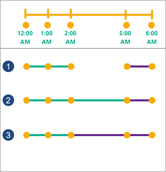
  Three examples of time splits on the same input points (yellow) are shown.

  Time split option	Description
  Five input points with a time and location	Five input points with the same identifier. The time of each point is marked below the dotted line. There is one split between 2:00 a.m. and 5:00 a.m. for all examples. Each track is split into two segments between the third and fourth points on the track. The first track is green and the second is purple. How the tracks are split is defined by the split type parameter.
  Gap	Example with a gap between the two points that are split. The first track ends at the third point and the second track starts at the fourth point. This is the default.
  Finish After	Example in which the track finishes after the split, at the fourth point. The second track starts at the fourth point. This option is available with ArcGIS Enterprise 10.9 or later.
  Start Before	Example in which the track splits before the split, at the third point. The second track starts at the third point. This option is available with ArcGIS Enterprise 10.9 or later.

• The following are examples of why it may make sense to define tracks using the split parameters and the field identifier parameter using an airline flight as an example:

  • An aircraft feature has aircraft ID, flight ID, pilot name, start time, and flight_maneuver fields. The flight_maneuver field represents whether the aircraft is on land, ascending, descending, or at a constant altitude.

    • Use the aircraft ID field as the identifier to see where each plane has traveled.

    • Use the aircraft ID and the flight ID fields as the identifiers to compare distinct routes.

    • Use the aircraft ID field and the time boundary of one year to examine the flights for each aircraft for a year at a time.

    • Use the pilot name, aircraft ID, and start time fields to view each pilot's flight.

    • Use the aircraft ID field as the identifier, and split distances farther than 1,000 kilometers, to determine new tracks, given that a 1,000-kilometer jump in measurements should not belong to the same track.

    • Use the aircraft ID field as the identifier and split using an expression when the value in the flight_maneuver field changes. For example, var flight_manuever = TrackFieldWindow("maneuver", -1, 1); flight_maneuver[0] != flight_maneuver[1] checks whether the current value in a track and the previous value match. If not, the track is split.

• Output tracks will return the fields used as track identifiers, the count of features within a track (count), the start and end time of each track (start_datetime and end_datetime), the duration of the track in milliseconds (duration), and any other optional statistics (formatted as statisticstype_fieldname).

• You can improve performance of the Reconstruct Tracks tool by doing one or more of the following:

  • Set the extent environment so that you only analyze data of interest.

  • Use the planar method instead of geodesic.

  • Don't apply a buffer.

  • Split your tracks using the Time Split, Time Boundary Split, Distance Split, or Split Expression parameters. The Time Boundary Split parameter will have the biggest performance gains.

  • Use data that is local to where the analysis is being run.

• This geoprocessing tool is powered by ArcGIS GeoAnalytics Server. Analysis is completed on GeoAnalytics Server, and results are stored in your content in ArcGIS Enterprise.

• When running GeoAnalytics Server tools, the analysis is completed on GeoAnalytics Server. For optimal performance, make data available to GeoAnalytics Server through feature layers hosted on your ArcGIS Enterprise portal or through big data file shares. Data that is not local to GeoAnalytics Server will be moved to GeoAnalytics Server before analysis begins. This means that it will take longer to run a tool and, in some cases, moving the data from ArcGIS Pro to GeoAnalytics Server may fail. The threshold for failure depends on your network speeds, as well as the size and complexity of the data. It is recommended that you always share your data or create a big data file share.

  Learn more about sharing data to your portal

  Learn more about creating a big data file share through Server Manager

• Similar analysis can also be completed using the following:

  • The Points To Line tool in the Data Management toolbox.

Parameters

• Dialog
• Python

Label	Explanation	Data type
Input Layer	The points or polygons to be reconstructed into tracks. The input must be a time-enabled layer that represents an instant in time.	Feature Set
Output Name	The name of the output feature service.	String
Track Fields	One or more fields that will be used to identify unique tracks.	Field
Method	Specifies the criteria that will be used to reconstruct tracks. If a buffer is used, the Method parameter determines the type of buffer. Geodesic—If the spatial reference can be panned, tracks will cross the date line when appropriate. If the spatial reference cannot be panned, tracks will be limited to the coordinate system extent and may not wrap. Planar—Planar buffers will be created.	String
Buffer Type	Specifies how the buffer distance will be defined. Field—A single field will be used to define the buffer distance. Expression—An equation using fields and mathematical operators will be used to define the buffer distance.	String
Buffer Field (Optional)	The field that will be used to buffer the input features. Field values are applied in the units of the spatial reference of the input unless you are using a geographic coordinate system, in which case they will be in meters.	Field
Buffer Expression (Optional)	The expression that will be used to buffer input features. Fields must be numeric, and the expression can include [+ - * / ] operators and multiple fields. Calculated values are applied in the units of the spatial reference of the input unless you are using a geographic coordinate system, in which case they will be in meters. In ArcGIS Enterprise 10.5 and 10.5.1, expressions are formatted as as_kilometers(distance) * 2 + as_meters(15). In ArcGIS Enterprise 10.6 or later, use Arcade expressions such as as_kilometers($feature.distance) * 2 + as_meters(15).	Calculator Expression
Time Split (Optional)	Features that are farther apart in time than the time-split duration will be split into separate tracks.	Time Unit
Summary Fields (Optional)	The statistics that will be calculated on specified fields. Value table columns: Field—Fields on which statistics will be calculated. Statistics—Statistics that will be calculated on specified fields. Count—The number of nonnull values. It can be used on numeric fields or strings. The count of [null, 0, 2] is 2. Sum—The sum of numeric values in a field. The sum of [null, null, 3] is 3. Mean—The mean of numeric values. The mean of [0,2, null] is 1. Minimum—The minimum value of a numeric field. The minimum of [0, 2, null] is 0. Maximum—The maximum value of a numeric field. The maximum value of [0, 2, null] is 2. Standard deviation—The standard deviation of a numeric field. The standard deviation of [1] is null. The standard deviation of [null, 1,1,1] is null. Variance—The variance of a numeric field in a track. The variance of [1] is null. The variance of [null, 1,1,1] is null. Range—The range of a numeric field. This is calculated as the minimum value subtracted from the maximum value. The range of [0, null, 1] is 1. The range of [null, 4] is 0. Any—A sample string from a field of type string. First—The first value of a specified field in a track. This option is available with ArcGIS Enterprise 10.8.1. Last—The last value of a specified field in a track. This option is available with ArcGIS Enterprise 10.8.1.	Value Table
Data Store (Optional)	Specifies the ArcGIS Data Store where the output will be stored. All results stored in a spatiotemporal big data store will be stored in WGS84. Results stored in a relational data store will maintain their coordinate system. Spatiotemporal big data store—Output will be stored in a spatiotemporal big data store. This is the default. Relational data store—Output will be stored in a relational data store.	String
Distance Split (Optional)	Features that are farther apart in distance than the distance split value will be split into separate tracks. This parameter is only available with ArcGIS Enterprise 10.6 and later.	Linear Unit
Time Boundary Split (Optional)	A time span to split the input data into for analysis. A time boundary allows you to analyze values within a defined time span. For example, if you use a time boundary of 1 day, starting on January 1, 1980, tracks will be split at the beginning of every day. This parameter is only available with ArcGIS Enterprise 10.7 and later.	Time Unit
Time Boundary Reference (Optional)	The reference time used to split the input data into for analysis. Time boundaries will be created for the entire span of the data, and the reference time does not need to occur at the start. If no reference time is specified, January 1, 1970, is used. This parameter is only available with ArcGIS Enterprise 10.7 and later.	Date
Split Expression (Optional)	An expression that splits tracks based on values, geometry or time values. Expressions that validate to true will be split. This parameter is only available with ArcGIS Enterprise 10.9 and later.	Calculator Expression
Split Type (Optional)	Specifies how the track segment between two features is created when a track is split. The split type is applied to split expressions, distance splits, and time splits. This parameter is only available with ArcGIS Enterprise 10.9 and later. Gap—No segment is created between the two features. This is the default. Finish After—A segment is created between the two features that ends after the split. Start Before—A segment is created between the two features that ends before the split.	String

Derived output

Label	Explanation	Data type
Output Feature Class	The output line or polygon tracks.	Feature Set

Environments

Output Coordinate System, Extent, Current Workspace

Special cases

Output Coordinate System

The coordinate system that will be used for analysis. Analysis will be completed in the input coordinate system unless specified by this parameter. For GeoAnalytics Tools, final results will be stored in the spatiotemporal data store in WGS84.

Licensing information

• Basic: Requires ArcGIS GeoAnalytics Server
• Standard: Requires ArcGIS GeoAnalytics Server
• Advanced: Requires ArcGIS GeoAnalytics Server

Related topics

• An overview of the Summarize Data toolset
• Find a geoprocessing tool
• Buffer expression examples for ArcGIS Enterprise 10.5 and 10.5.1