How Huff equal probability trade areas work
The Generate Huff Equal Probability Trade Areas tool creates trade areas around point locations, shaped by two factors:
Distance as a dissuasive factor
Attractiveness as a persuasive factor
Does the attractiveness of a store—whether that is defined by product prices, availability of parking, or other desirable factors—outweigh the effects of the distance-decay function, which posits that location desirability decreases as distance increases? The tool uses the principles of the Huff model to express and resolve the tension between distance and attractiveness, drawing trade areas that indicate the sphere of influence of each store relative to each other.
To learn more about the calculations used in the Huff model, see How Huff Model works.
Parameters
The following sections provide explanations of how different parameters affect the tool's output.
Distance factors
Around each location, there is always an area where that store is dominant, based purely on distance. Beyond the most proximate area, attractiveness determines the gravitational pull towards particular stores. In a situation where the attractiveness of all stores is equal, trade areas are drawn as Thiessen polygons, based on distance alone.
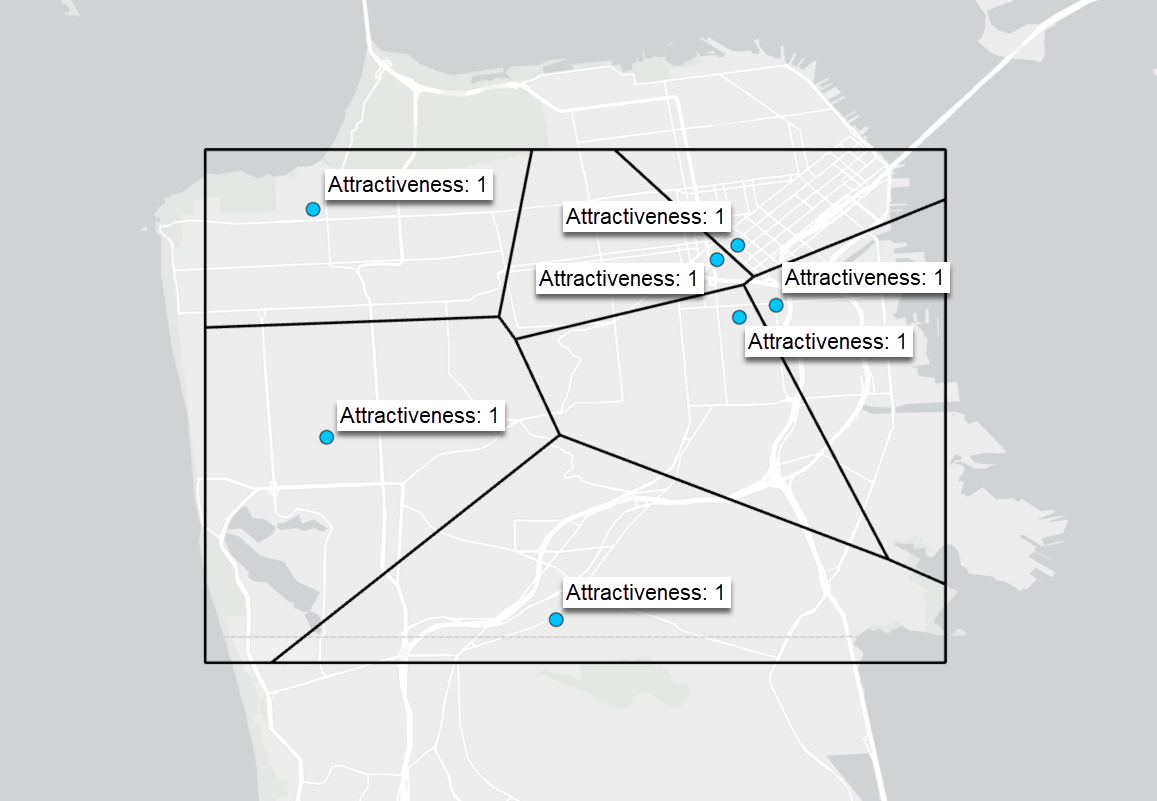
In this situation, a line is drawn halfway between two competing locations and provides a basic approach to drawing boundaries between stores.
Attractiveness factors
The attractiveness of a location can defray the effects of distance, creating larger trade areas around more attractive stores. You can combine multiple attractiveness factors, each with their own exponent. The higher the exponent, the more that factor influences the result.
In the example below, consider the store clusters in the northeast, where stores with lower attractiveness generate smaller trade areas compared to nearby stores with higher attractiveness.
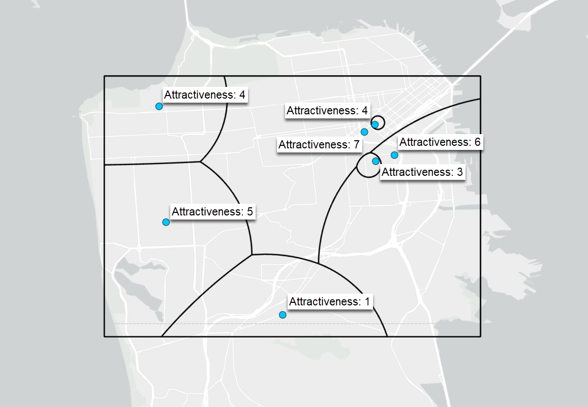
Attractiveness can be any characteristic of a location that impacts its appeal to consumers or patrons. The variable used to calculate attractiveness must be a numeric field contained in the input point layer, such as sales volume or store square footage.
Distance and attractiveness exponents
The distance exponent and the attractiveness exponent determine the strength of distance and attractiveness, respectively, on the trade areas. A high distance exponent means that distance will have a strong impact on dissuading people from visiting a store; a high attractiveness exponent means that attractiveness will have a strong impact on persuading people to visit a store, and so on.
Distance exponent—Always a negative number. A more negative value strengthens the dissuasive effect of distance and produces more localized trade areas.
Attractiveness exponent—Usually a positive number. A higher value amplifies the influence of attractiveness, allowing stronger stores to dominate more distant territory. There are also situations where the attractiveness exponent could be a negative value, to reflect a field that has a negative impact on attractiveness. For example, if the attractiveness variable is the number of complaints against a store, then the exponent can show the severity of this as a non-attractive factor: the more complaints, the lower the attractiveness.
The higher (more negative) the distance exponent, the more localized the results. A higher (more positive) attractiveness exponent may suggest that bigger stores dominate more strongly. You may want to test multiple values and compare outputs visually.
Calibrated Huff models
Using a calibrated Huff model (a .huffmodel file) when generating Huff equal probability trade areas allows you to apply distance and attractiveness exponents that have been built using your own customer data. By default, the Use Existing Huff Model Calibration parameter is set to use custom exponents that you define within the tool. When you instead use an existing Huff model calibration file, the distance and attractiveness exponents are automatically populated from the file.
To learn more about calibrating a Huff model, see the following:
Geometric concepts
There are two spatial-geometric principles that underlie the trade areas created by the Generate Huff Equal Probability Trade Areas tool: multiplicatively weighted Voronoi diagrams and Apollonius circles.
Multiplicatively weighted Voronoi diagrams
Multiplicatively weighted Voronoi (MW-Voronoi) diagrams depict regions around points by accounting for both regional distance and the weight of the points the regions are built around. In the case of this trade area tool, the weight is the attractiveness of the location (or the sum of multiple attractiveness variables) added from the input point layer.
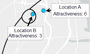
Consider that you have two locations on the map, location A and location B.
MW-Voronoi Formula
The formula for creating MW-Voronoi using this tool is as follows:
Terms
\(x\): Any point in the map extent
\(A\) and \(B\): Point locations in the map extent
\(WD\): Weighted distance
\(ED\): Euclidean distance
\(W\): Weight (in this case, attractiveness)
Weighted distance is the Euclidean distance divided by the location’s weight. Thus, the larger a location’s weight, the smaller its weighted distance, effectively making the location “closer.” So, for the trade area around location A, we include all points where the weighted distance to A is less than or equal to the weighted distance to B. This creates a larger trade area for location A than for location B.
Apollonius circles
Apollonius circles, in the context of this trade area tool, create trade area boundaries at a fixed distance ratio from two sources. This geometric property is what transforms the straight-edged, square-like shapes of ordinary Thiessen polygons into the smooth, curved trade-area boundaries characteristic of the tool. A store with twice the weight of its neighbor will claim territory whose boundary is an arc of an Apollonius circle, expanding its reach in a natural, gravity-like manner.
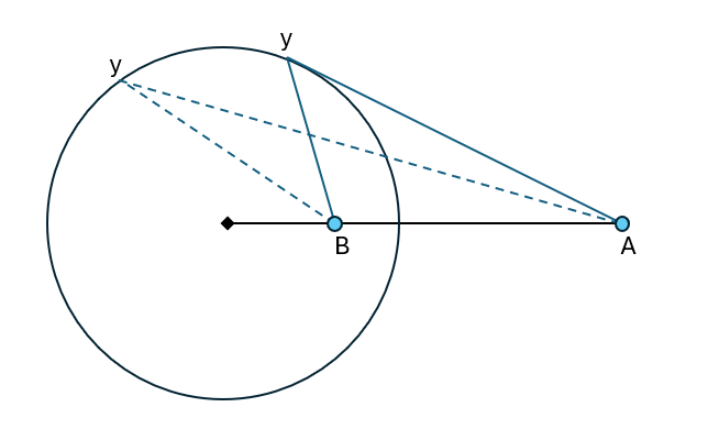
Consider the previous example, with location A and location B. For this tool, the \(k\) constant is the ratio of the attractiveness variables. So in this case, \(k\) = 6/3.
References
The following articles informed the design of this tool:
Huff, D.L. (1973). "The delineation of a national system of planning regions on the basis of urban spheres of influence." Regional Studies, 7, 323-329.
Mu, L. (2004). "Polygon Characterization With the Multiplicatively Weighted Voronoi Diagram." The Professional Geographer, 56(2), 223–239. https://doi.org/10.1111/j.0033-0124.2004.05602007.x
Note:
This tool uses the azimuthal equidistant map projection. To learn more, see Azimuthal equidistant.
Suggested exponents
Understanding how distance and attractiveness shape the trade areas for different industries is crucial to creating accurate trade areas using this tool. The following examples are intended as starting points for your own analyses.
|
Industry |
Exponents |
Notes |
|---|---|---|
|
Convenience Goods (Everyday essentials such as groceries, pharmacy, or fast food) |
|
Best for customers who prefer nearby options and shop frequently. Large stores still matter, but proximity dominates. Expected result: Small, localized trade areas. |
|
Shopping Goods (Apparel, home goods, electronics, or department stores) |
|
Best for comparison shopping where store size, selection, and appeal matter more. Expected result: Medium-to-large trade areas with clear winners among bigger stores. |
|
Specialty/Destination (Retail furniture, appliances, luxury goods, or flagship stores) |
|
Best for infrequent, high-value purchases where customers are willing to travel for the right store. Expected result: Very large, overlapping trade areas dominated by high-attractiveness locations. |
|
Mixed Urban Convenience (Urban supermarkets or convenience stores in dense cities) |
|
Best for walkable or transit-oriented areas with good public transport. Expected result: Compact but competitive trade areas; size still provides an advantage. |
|
Big-Box/Regional Power Centers (Large-format retailers, malls, outlet centers) |
|
Best for regional draws where customers drive longer distances for variety and scale. Expected result: Very broad trade areas with strong hierarchy based on store size/sales volume. |
Attractiveness variable examples
The following are variables that can be used (alone or in combination) to quantify attractiveness, with an associated exponent range.
|
Variable |
When to use |
Exponent range |
Notes |
|---|---|---|---|
|
Number of employees |
Labor-intensive retail or service businesses |
1.0 to 3.0 |
Good proxy for store capacity and service level |
|
Product assortment/SKU count |
Fashion, electronics, home goods |
1.5 to 4.0 |
Captures variety and selection power |
|
Customer ratings/Review score |
Any retail with online reviews |
2.0 to 5.0+ |
Strong effect when quality perception matters |
|
Parking spaces |
Auto-oriented locations |
0.8 to 2.5 |
Very relevant for suburban big-box stores |
|
Amenities score |
Malls, lifestyle centers |
1.5 to 3.5 |
Includes restaurants, playgrounds, events, etc. |
|
Brand strength/Flagship status |
National chains versus independents |
2.0 to 4.0 |
Can be a binary or scaled variable |
|
Public transit accessibility |
Urban or transit-rich areas |
1.0 to 3.0 |
Combine with distance exponent |
|
Price index/value perception |
Discount versus premium retailers |
1.5 to 3.5 |
Works well for price-sensitive segments |
|
Open hours/accessibility hours |
24-hour or extended-hour stores |
0.8 to 2.0 |
Useful for pharmacies or grocery |
|
Store age/renovation status |
Newer or recently remodeled stores |
1.0 to 2.5 |
Signals modernity and investment |