How the Multicriteria Overlay tool works
The Multicriteria Overlay tool combines multiple input rasters into a single output raster using various Multicriteria Decision Analysis (MCDA) overlay methods. MCDA is a structured approach used in spatial decision-making tasks, such as site selection, suitability modeling, mapping risk, and prioritizing areas for planning.
The method involves two main steps. The first is transforming all criteria to a common scale. The second is weighting and combining the transformed criteria to produce an output.
This tool performs the second step, that being applying an overlay method that fits your analysis goals.
Primary considerations
The following are the main considerations when performing a multicriteria overlay analysis:
Prepare and transform the input rasters
Choose an overlay method
Assign the weights for input rasters
More details on these considerations are provided below. Following that are additional sections that describe the mathematical calculations and potential applications for each method.
Prepare and transform the input rasters
Choose input rasters that are directly related to the multicriteria problem and can be quantified. Each raster should measure a single criterion. Because raster datasets often vary in units, value ranges, and whether higher or lower values indicate greater suitability, the rasters should first be transformed onto a common scale so they can be combined. Transforming rasters ensures that no single criterion disproportionately influences the results and the suitability values are interpreted consistently.
Consider as an example a habitat suitability analysis. In order to capture an animal's requirements for food sources, you might use a raster of land cover type and a raster that records the proximity to streams. To provide security, a raster that records the distance away from buildings and a slope raster can help to find areas with minimal potential from human contact. Use the Reclassify tool to assign suitability values to the different land-use types based on the habitat preferences of the study animal. For rasters that represent continuous criteria, use the Rescale by Function tool to transform them onto a common suitability scale.
Choose an overlay method
There are many different overlay methods available, and they each have different strengths and requirements. Study each of the overlay methods then select one that best fits your analytical objectives and the behavior you want to model.
Assign the weights for input rasters
Weights must be assigned that reflect the relative importance of each input in meeting the analytical objectives.
The weights can be based on expert consultation or derived from statistical analysis. Since the results of the analysis can be significantly influenced by the weighting process, it is important to ensure that weight values are justified.
Weighted sum
Use the Weighted sum option of the Overlay Method parameter when tradeoffs among input rasters are acceptable. A high value in one raster can compensate for a low value in another, producing a result that represents the overall combined performance or suitability across all input criteria.
Formula
For this method, the cell values from each input raster are multiplied by their corresponding weight. The results are added together to create the output raster.
Expressed as a formula, the output value for each location is calculated as:
\(OutRas = (Ras1 \times Weight1) + (Ras2 \times Weight2) + \ldots + (RasN \times WeightN)\)
Example
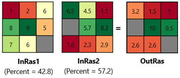
The illustration below shows the result of applying the formula to two input example rasters with a different weight factor applied. These inputs will be used in the examples for all the other methods.
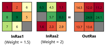
Consider the upper left cell. For InRas1, the location has a cell value of 1. Multiplying it by the weight of 1.5 results in a value of 1.5. For InRas2, the location has cell value of 6.5, so the result of multiplying it by the weight of 2 is 13.
Adding the values 1.5 and 13 results in an output cell value of 14.5 for that location.
Potential applications
Applications for this method include:
Wind farm siting: In a wind farm site selection project, use this method to aggregate several criteria into a single suitability map. The method can capture how having excellent wind resources can outweigh conditions, such as moderate slope, based on their assigned importance.
Winery plantation planning: In vineyard site planning, the weighted sum method is used to combine natural climate conditions, cost-related factors, and soil properties into a final suitability score. High climate and soil suitability can offset less favorable cost conditions considering long-term profits.
Weighted geometric mean
Use the Weighted geometric mean option of the Overlay Method parameter for analyses where all input rasters have relatively high values.
The calculation is based on multiplication, so a low value in any input raster will proportionally reduce the final suitability and cannot be compensated for by higher values in other rasters. It is often chosen to maintain the influence of low values as a limiting factor, while still incorporating contributions from other inputs. The exponential nature of the weights allows control over how strongly low values affect the outcome.
Formula
For this method, for each location the cell values from each input rasters are raised to the power of their corresponding weight. The results are multiplied, then the product is raised to the power of the sum of all the weights.
Expressed as formulas, first the sum of all the weights is calculated:
\(Weights\_sum = Weight1 + Weight2 + \ldots + WeightN\)
Next, all of the input cell values are raised to the power of their associated weight, and the product of those values is calculated:
\(Values\_product = Ras1^{Weight1} \times Ras2^{Weight2} \times \ldots \times RasN^{WeightN}\)
The final output value for each location is calculated by raising the product of the weighted values to the inverse sum of all the weights.
\(OutRas = Values\_product^{(1 / Weights\_sum)}\)
Example
The illustration below shows the result of applying this formula to the same inputs and the same weights used in the weighted sum method.
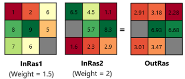
For InRas1, the upper left cell of value 1 is raised to the power of the weight. The result of 11.5 = 1.
For InRas2, the weight causes the input cell value of 6.5 to be raised to the power of 2, which results in a value of 42.25.
The product of 1 and 42.25 is 42.25. The sum of the weights is 1.5 + 2 = 3.5.
The final output for that location is 42.25(1 / 3.5) ≈ 2.91
Potential applications
Applications for this method include:
Habitat suitability index: In habitat modeling, multiple criteria—such as water quality, temperature, and light availability—are combined using a weighted geometric mean so a site cannot score highly unless all essential habitat conditions are favorable.
Aquaculture site suitability and yield estimation: In farming site evaluation, several environmental quality criteria are aggregated with a weighted geometric mean so overall suitability drops sharply when any critical environmental condition is poor.
Maximum
Use the Maximum option of the Overlay Method parameter when the input rasters can substitute for one another and you want the result to reflect the strongest advantage or highest value at each cell rather than overall balance. A cell receives a high output value when at least one of the weighted input values has a high value, even if the other weighted input values are low.
Formula
For each input cell, the tool will assign the largest value among the weighted input rasters at that location.
The formula for calculating the maximum of the weighted input vales for each location:
\(OutRas = Maximum\{(Ras1 \times Weight1), (Ras2 \times Weight2), \ldots, (RasN \times WeightN)\}\)
Example
The result of applying this formula to the same inputs and the same weights are:
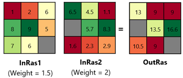
For InRas1, the upper left cell value of value 1 is multiplied by the weight of 1.5, resulting in a value of 1.5. For InRas2, the cell value of 6.5 is multiplied by the weight of 2, which results in 13.
This method returns the largest of the two weighted values, so the output value will be 13.
Potential applications
Applications for this method include:
Mineral exploration: In cobalt prospectivity mapping, multiple criteria are combined using the Maximum overlay method so a cell is highlighted if any one indicator strongly supports mineral potential.
Wireless coverage mapping: In radio network planning, signal strength rasters from multiple base stations are combined using the Maximum overlay method so each cell represents the strongest available coverage at that location.
Minimum
Use the Minimum option of the Overlay Method parameter when you want the result to reflect the most limiting factor at each cell. A cell will receive the lowest value of the weighted input rasters, even if other weighted inputs are high.
Formula
For each input cell, the tool will assign the smallest value among the weighted input rasters at that location.
The formula for calculating the minimum of the weighted input vales for each location is:
\(OutRas = Minimum\{(Ras1 \times Weight1), (Ras2 \times Weight2), \ldots, (RasN \times WeightN)\}\)
Example
The result of applying this formula to the same inputs and the same weights are:
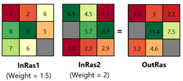
The upper left cell value of InRas1 is 1, and multiplying by the weight of 1.5 resulting in the value 1.5. For InRas2, the cell value of 6.5 is multiplied by the weight of 2, which results in 13.
This method returns the lowest of the two weighted values, so the output value will be 1.5.
Potential applications
Applications for this method include:
Habitat suitability: In habitat modeling, food and water availability, landuse type, and human disturbance are all considered key limiting factors. They are combined using the Minimum overlay method so a cell is rated low if any essential habitat condition are poor.
Solar farm siting with multiple submodels: Three submodels suitability maps are created for solar resource suitability, accessibility, and environmental impact. Because solar resource is treated as a limiting factor, the Minimum method is used to derive the final suitability, ensuring that locations with poor solar potential remain low in suitability even if other conditions are favorable.
Weighted overlay
Use the Weighted Overlay option of the Overlay Method parameter when you want each criterion to contribute to the result as a percentage of the final output. The weight values for this option must be specified as percentage values, and need to sum to 100. Each value specified for the Percent parameter value means how strongly each criterion influences the final output relative to the other criteria.
The combined result is then rescaled to an evaluation range defined by the From Scale and To Scale parameters, such as 0 and 1 or 1 and 10. This ensures that the output raster values stay within a consistent range, making it easier to directly compare results generated from different input criteria or weighting setting.
Formula
For each location, corresponding cell values in each input raster are multiplied by the value provided for the Percent option. All the weighted values are added together. That result is then scaled to the defined output range.
The output value for each location is calculated as
\(CombinedValue = (Ras1 \times Percent1) + (Ras2 \times Percent2) + \ldots + (RasN \times PercentN)\)
Then the weighted summed output is rescaled using the formula below:
\(OutRas = {FromScale} + ({CombinedValue} - {CombinedValue}_{\min}) \cdot \large \frac {ToScale - FromScale}{CombinedValue_{\max} - CombinedValue_{\min}}\)
Example
The result of applying this formula follows. The output scale chosen for this example is 1-10.
For InRas1 the upper left cell of value 1 multiplied by the decimal percentage 0.428 = 0.428. For InRas2, the cell value of 6.5 multiplied by the decimal percentage 0.572 = 3.718.
The sum of these two values is 4.146.
The tool then performs these calculations for all 9 input locations. The resulting minimum value is 3.197, and the maximum value is 7.112.
Applying these values to the formula results in the following final output value for this location:
\(\begin{aligned}OutRas &= 1 + (4.146 - 3.1972) \cdot \frac{10 - 1}{7.1124 - 3.1972} \\ &= 3.2\end{aligned}\)
Potential applications
Because this method uses an additive combination, its applications are similar to Weighted Sum, but the weights are expressed as percentages and the final values stay within the specified range.
Ordered weighted averaging
Use the Ordered weighted averaging option of the Overlay Method parameter when you want to emphasize the high value criterion to low value criterion, or when you want to explore how sensitive results are to different levels of tradeoff and compensation
Unlike methods that apply fixed weights to fixed criteria positions, Ordered weighted averaging (OWA) first sorts the weighted criterion values at each cell from highest to lowest. It then applies a separate set of order weights to the ranked values that control how much influence the best, middle, or worst criterion has.
By changing the order weights, you can shift the result from minimum-like behavior (where low criterion values strongly limit the output) to maximum-like behavior (where high criterion values have the most influence). Use the ability to customize the order weight settings to control how high values can offset low values across the criteria.
Using certain settings for the weights can approximate the results of different overlay methods.
If you assign an order weight of 1 to the highest weighted criterion and 0 to all others, OWA behaves like the Maximum method.
If you assign an order weight of 1 to the lowest weighted criterion and 0 to all others, OWA behaves like the Minimum method.
If you give equal order weights to all ranked values, OWA behaves like a Weighted sum method, where criteria contribute evenly to the result.
There are two ways to specify the order weights. When the Order Weights Method parameter value is set to the Custom option, you can enter the weights manually. Choose the Quantifier-guided option to derive them automatically.
For the Quantifier-guided option, an Orness value is used to control the shape of the order weights. Orness describes how optimistic the overlay is. Higher values give more influence to the highest-ranked weighted input raster value. This produces a behavior similar to the Maximum option of the Overlay Method parameter. Lower values give more influence to the lowest-ranked weighted input raster value. This produces a behavior similar to the Minimum option of the Overlay Method parameter.
Formula
For each input raster, multiply every cell value by the value of the defined weight for that input. Next, for each cell location, rank the weighted values from highest to lowest. Multiply the order weights based on the sorted values, then sum them together to produce the final output value for that cell.
First, calculate the weighted input value for each input location.
\(WeightedInput1 = Ras1 \times Weight1\)
\(WeightedInput2 = Ras2 \times Weight2\)
\(\ldots\)
\(WeightedInputN = RasN \times WeightN\)
Next, the weighted values will be ranked from highest to lowest.
\(Ranked\_values = \{Rank1(WeightedInput1), Rank2(WeightedInput2), \ldots, RankN(WeightedInputN)\}\)
A list of order weight values will either be provided as input or can be generated by the tool.
\(List\ of\ weight\ values = \{RankWeight1, RankWeight2, \ldots, RankWeightN\}\)
The order weight values are multiplied by the ranked weighted values and then summed together to provide the value for that cell location in the final output raster.
\[ \begin{array}{l} OutRas = (RankWeight1 \times Rank1(WeightedInput1)) + (RankWeight2 \times Rank2(WeightedInput2)) \\ \phantom{OutRas = {}} + \ldots + (RankWeightN \times RankN(WeightedInputN)) \end{array} \]
Example
Applying this method to the example inputs results in the following output.
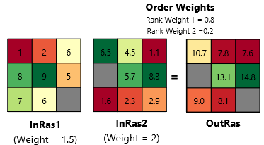
For InRas1, the value of the upper left cell location is multiplied by the weight, and the result of 1 x 1.5 = 1.5. For InRas2 the result is 6.5 x 2 = 13
The weighted values for this location ranked from highest to lowest are 13 and 1.5.
The provided order weights 0.8 and 0.2 are applied to the ranked values. For InRas2 the result is 13 x 0.8 = 10.4. For InRas1, the result is: 1.5 x 0.2 = 0.3.
The sum of these two values is 10.4 + 0.3 = 10.7.
Potential applications
Applications for this method include:
Integrated agricultural planning: By applying different combinations of order weights, you can compare an output suitability map that:
Enforces strict limiting criteria for reliable long-term production.
Highlights high-potential opportunities for near-term expansion.
Reveals balanced strategies that emphasize moderately suitable areas, avoiding extremes, which can be useful for risk-averse planning.
Landslide susceptibility mapping: You can adjust the order weights to control how much trade-off is allowed among landslide factors, such as slope, rainfall, geology, and land cover.
This makes it possible to compare susceptibility maps that:
Apply a strict, limiting factor rule with little or no trade-off.
Use a more permissive rule where strong factors can have greater influence.
Test intermediate strategies that allow partial compensation among criteria.
Ideal point solutions (TOPSIS)
Use the Ideal point solutions (TOPSIS) option of the Overlay Method parameter when you want a balanced compromise solution. This option identifies locations that simultaneously favor being near desirable conditions and are far from undesirable conditions. Unlike the others, this method can optimize more than one factor.
A positive ideal point (most preferred) and a negative ideal point (least preferred) for each input raster needs to be provided.
They do not need to be the minimum and maximum of the input raster. For example, if an aspect raster is an input and south-facing slopes are preferred, you can set 180 as the positive ideal value and 0 as the negative ideal value.
They do not need to be within the input raster value ranges. For example, when creating an air quality index, one important criterion is PM2.5 concentration (lower is better). In your dataset, neighborhoods in the city range from 18 μg/m³. If you use the WHO guideline 5 μg/m³ as the ideal value, that ideal point is below the minimum in the input raster range. TOPSIS can still use it as a reference to measure how close each neighborhood is to the ideal, even if no location in the city currently meets that standard.
Formula
For the TOPSIS algorithm, a positive ideal point (highest preferred) and a negative ideal point (lowest reference) for each input raster is identified in the units of the input raster. Each input raster is first standardized by dividing every cell value by the square root of the sum of squared values in that raster, placing all rasters on a common scale. The standardized raster is then multiplied by its assigned weight. Next, the distance from each cell to the positive ideal solution and the negative ideal solution is calculated. The final output is determined by the relative closeness coefficient, which is calculated from each cell's distance to the positive ideal solution and the negative ideal solution. In general, higher values represent more preferred cells because they are relatively closer to the positive ideal solution and relatively farther from the negative ideal solution.
Each input raster and the ideal point values are standardized using the formula below to make the values from different rasters comparable.
\(\large r_{ij} = \large \frac {\large x_{ij}}{\large \sqrt{\sum_{i=1}^{n} x_{ij}^2}}\)
where:
\(x_{ij}\) is the value of cell \(i\) for input raster \(j\). It also represents ideal point values for that input raster \(j\).
\(n\) is the number of all valid cells in the analysis extent.
\(r_{ij}\) is the normalized value of cell \(i\) for input raster \(j\).
At each cell, TOPSIS then computes the cell's distance to the standardized positive ideal solution and to the standardized negative ideal solution using the selected Distance Method parameter value. Then, the input raster weights are applied to the distance calculation so that more important criteria contribute more to the positive and negative distances.
The Distance Method parameter provides two options for calculating distance: Euclidean distance and Manhattan distance.
For Euclidean distance, the weighted distances are computed as:
\(\large d_{i}^{+} = \sqrt{\sum_{j=1}^{m} w_{j}(r_{ij} - r_{j}^{+})^{2}}\)
\(\large d_{i}^{-} = \sqrt{\sum_{j=1}^{m} w_{j}(r_{ij} - r_{j}^{-})^{2}}\)
For Manhattan distance, the weighted distances are computed as:
\(\large d_{i}^{+} = \sum_{j=1}^{m} w_{j}\left|r_{ij} - r_{j}^{+}\right|\)
\(\large d_{i}^{-} = \sum_{j=1}^{m} w_{j}\left|r_{ij} - r_{j}^{-}\right|\)
where:
\(d_{i}^{+}\) is the weighted distance from cell \(i\) to the standardized positive ideal solution.
\(d_{i}^{-}\) is the weighted distance from cell \(i\) to the standardized negative ideal solution.
\(r_{ij}\) is the standardized value of cell \(i\) for input raster \(j\).
\(r_{j}^{+}\) is the standardized positive ideal value for raster \(j\).
\(r_{j}^{-}\) is the standardized negative ideal value for raster \(j\).
\(m\) is the number of input rasters.
Finally, the two distances are converted to a single closeness score using the formula below:
\(OutRas = \frac{\large d_i^{-}}{\large d_i^{+} + d_i^{-}}\)
Example
Applying this method to the example inputs results in the following output.
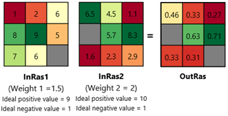
The first step is to standardize the cell values. Since each raster has one NoData cell, those two locations will be excluded in the calculation.
For raster 1, the standardization factor is:
\(\sqrt{1^2 + 2^2 + 6^2 + 8^2 + 9^2 + 5^2 + 7^2 + 6^2} \approx 17.205\)
So for the upper left cell of raster 1, the normalized value is:
\(r_{1} = \frac {1}{17.205} = 0.058\)
For raster 2, the standardization factor is:
\(\sqrt{6.5^{2} + 4.5^{2} + 1.1^{2} + 5.7^{2} + 8.3^{2} + 1.6^{2} + 2.3^{2} + 2.9^{2}} \approx 13.467\)
So for the upper left cell of raster 2, the normalized value is:
\(r_{2} = \frac{6.5}{13.467} = 0.483\)
Standardize the ideal point values using the same factors.
For raster 1, the ideal positive and negative values are 9 and 1 respectively.
\(r_{1}^{+} = \frac{9}{17.205} = 0.523 \qquad r_{1}^{-} = \frac{1}{17.205} = 0.058\)
For raster 2, the ideal positive and negative values are 10 and 1 respectively.
\(r_{2}^{+} = \frac{10}{13.467} = 0.742 \qquad r_{2}^{-} = \frac{1}{13.467} = 0.074\)
Compute the distance to the positive ideal and negative ideal with weights applied.
For ideal positive distance:
\(d^{+} = \sqrt{1.5 \times (0.058 - 0.523)^2 + 2 \times (0.483 - 0.742)^2} = 0.678\)
For ideal negative distance:
\(d^{-} = \sqrt{1.5 \times (0.058 - 0.058)^2 + 2 \times (0.483 - 0.074)^2} = 0.578\)
Compute the final TOPSIS score
\(Out_{cell} = \frac{0.578}{0.679 + 0.578} = 0.460\)
Potential applications
Applications for this method include:
Sustainable urban development: Use TOPSIS when you want to identify areas that are most suitable for sustainable urban development based on multiple indicators, such as access to public transit, vegetation coverage, and pollution exposure. The method compares each location to an ideal set of desirable conditions and to an opposite set of undesirable conditions. Areas closer to the ideal solution and farther from the negative ideal solution receive higher suitability values, helping planners identify locations that better support sustainable development goals.
Solid waste disposal site suitability: Use TOPSIS to combine multiple criteria to site a solid water disposal location. Favorable conditions—sites that are environmentally safer, technically feasible, and less likely to affect nearby communities—define the positive ideal solution, while unfavorable conditions—locations close to settlements or water bodies, or areas with unsuitable terrain/land use—define the negative ideal solution. TOPSIS helps you identify sites that are simultaneously closest to the desired disposal conditions and farthest from unsuitable conditions.