How Calculate Location Quotients works
The Calculate Location Quotients tool computes the relative concentration of a variable at a location to a benchmark concentration by calculating a ratio of ratios. The benchmark may be the concentration of the entire feature class, a provided reference rate, or the concentration of a subset of features that share a trait. Location quotients help answer the question: how does the concentration of a variable at a location compare to a broader region? A location quotient greater than one indicates that the local share or concentration exceeds the benchmark; a value less than one signifies the local share falls short of the benchmark; and a value of one indicates the local share is identical to the benchmark.
Potential applications
Location quotients are useful in a variety of fields. The following are some potential applications of the tool:
Industry specialization- Compare employment in specific industries in a region to employment in those same industries across a broader region. For example, employment in manufacturing in US counties relative to employment in manufacturing across the entire US.
Crime specialization- Compare types of crime in an area to types of crime in an overall study area. For example, compare the relative level of traffic stops resulting in warnings across census tracts.
Demographics- Identify regions where specific populations, such as college students or families with children, are disproportionately concentrated.
Public health- Identify areas with higher populations of at-risk individuals such as smokers or those with chronic medical conditions.
Business and retail - Answer questions such as the following:
Where are ice cream shops unusually prevalent?
Which counties specialize in wineries?
Where are retail sales in footwear disproportionally high?
Background
Location quotients compare the local share of a variable to a regional or reference share by calculating a ratio of ratios. Location quotients are calculated as follows:
where \(E_{i,r}\) is the analysis variable at region \(r\), \(E_r\) is the total variable at region \(r\), \(E_{i,R}\) is the sum of the analysis variable across the selected study area, and \(E_R\) is the sum of the total variable across the selected study area. The numerator, \(\frac{E_{i,r}}{E_r}\), is the local share. For example, if the analysis variable is employment in manufacturing, the total variable is employment, and \(i\) is the feature Washington state, then the numerator represents the share of total employment in Washington state that is accounted for by employment in manufacturing.
Note:
The analysis variable value, at a location, is a subset of the total variable value. The analysis variable value can never exceed the total variable value.
The denominator, \(\frac{E_{i,R}}{E_R}\), is the reference or benchmark share. In the example, this is the total employment in the US that is accounted for by employment in manufacturing. The Benchmark Type parameter allows you to specify whether this benchmark value is calculated using all the features (Global (all features)), a subset of the features (Stratified (case-field)), or a provided value (Reference rate).
The location quotient is a ratio of these two ratios. It compares the concentration of a variable in a region to a broader region. In our example, the concentration of manufacturing employment in Washington state is compared to the concentration of manufacturing employment across the US.
Interpretation
Location quotients measure the relative concentration of a variable in a local area compared to its concentration in a broader benchmark region. Location quotients have a lower bound of zero and no upper bound. The relationship of a location quotient to 1 can be interpreted as follows:
Less than 1—The variable is less concentrated locally than in the reference region. For example, a location quotient of 0.5 means the local share is half that of the reference share. If nationally 30% of housing is renter-occupied, a county with a location quotient of 0.5 has only 15% of its housing occupied by renters.
Equal to 1—The local concentration matches the concentration in the reference region.
Greater than 1—The variable is more concentrated locally than in the reference region as a whole. A county with a location quotient of 2 has twice the prevalence of renter-occupied housing compared to the national rate. Extending our previous example, this county would have 60% renter-occupied housing.
Limitations
Location quotients are valuable descriptive statistics; however, they come with the following limitations and challenges:
Small numbers can produce unstable results. If the total variable is small, a relatively minor change in the analysis variable can result in extreme location quotient values. Consider a small town with a single manufacturing employer. This town may appear highly specialized in manufacturing even though the total number of employees is quite small.
Each analysis variable must be a subset of the total variable. You cannot use the tool to evaluate the relative density of two separate variables. For example, you cannot use the tool to compare the density of trees in a county to the density of trees in a state. In this scenario, the analysis variable (number of trees) is not a subset of the total variable (area).
Location quotients measure relative concentration, not magnitude. A high location quotient does not necessarily correspond to a large amount. For example, one area may have 500 manufacturing jobs and a location quotient of 3.0, while another has 10,000 manufacturing jobs and a location quotient of 0.8.
Tool inputs
The tool includes several parameters to select analysis variables and fine tune the local share and benchmark share values.
Analysis variables
The Analysis Variables parameter allows you to specify the analysis variable of interest. You can select a single variable or multiple variables if your data contains related variables. For example, if your total variable field represents employment and your data includes employment in several industries (manufacturing, health, education, etc.) then you can select multiple Analysis Variables values. Every analysis variable must be a subset of the total variable; the sum of all the analysis variables cannot exceed the total variable value.
Comparing multiple related location quotients at a single location allows you to answer the following:
Is there a dominating category, industry, or variable at a location?
What are the most (or least) prevalent categories, industries, or variables at a location?
Benchmark type
The Benchmark type parameter determines how the benchmark is calculated. The parameter supports the following options:
Global (all features)—Every feature in the feature class will be included in the benchmark value.
Stratified (case-field)—Allows you to specify a case field in the feature class that will be used to separate the features. Features that have the same value in the case field will be grouped. Each group will have a separate benchmark value calculated using the features in its group. For example, if the Case Field value is a state field then features in the same state will be grouped and each state will have a separate benchmark value.
Reference rate—Allows you to enter a reference rate for each analysis variable. For example, if you know the national rate of renter occupied housing however you only have data for census tracts in a single state, then you can select the Reference Rate option for the Benchmark Type parameter and set the Rate value to the national rate.
Location quotient type
The Location Quotient Type parameter determines how a location’s local share will be calculated.
Location quotient
The Location Quotient option uses a feature’s analysis variable and total variable value to calculate its local share.
where \(r\) is the local region, \(E_{i,r}\) is the analysis variable at region \(r\), and \(E_r\) is the total variable at region \(r\). The location quotient is then calculated as follows:
where \(E_{i,R}\) is the sum of the analysis variable across the selected study area and \(E_R\) is the sum of the total variable across the selected study area.
Focal location quotient
The Focal Location Quotient option uses the analysis variable and total variable values of each feature’s neighborhood to calculate its local share. The Neighborhood Type parameter assigns each feature a neighborhood and neighbor weights. By default, the weights of the focal feature and neighbors are all 1. For even greater control over neighbor and neighbor weight selection, use Neighborhood Explorer or the Generate Spatial Weights Matrix tool to create a .swm file. The focal local share of feature \(i\) is calculated as follows:
where \(r\) is the local region, \(n\) is the total number of neighbors, \(r'\) are the neighbors of feature \(r\), \(w_{rr'}\) is the weight of neighbor \(r'\), \(E_{i,r'}\) is the analysis variable value of neighbor \(r'\), and \(E_{r'}\) is the total variable value of neighbor \(r'\). The focal location quotient option spatially smooths location quotients and may be appropriate when features have small total variable values. The focal location quotient of region \(r\) (\(FLQ_{i,r}\)) is then calculated as follows:
where \(E_{i,R}\) is the sum of the analysis variable across the selected study area and \(E_R\) is the sum of the total variable across the selected study area.
Tool outputs
The tool produces several outputs, including an output feature class, charts, and pop-ups.
Output features or table
The output feature class or table will include a field for each analysis variable, the total variable, the benchmark type selected, the location quotient of each analysis variable, and the benchmark value of each analysis variable.
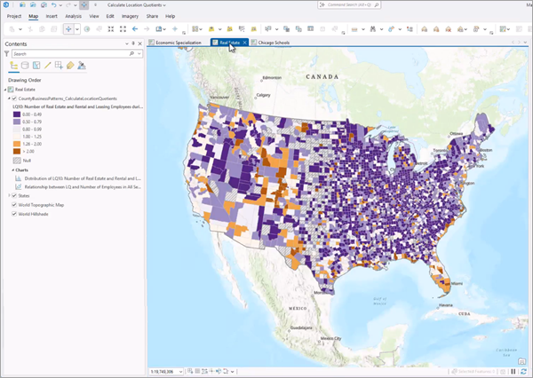
The default output symbology layer visualizes the first location quotient with a diverging color scheme.
Note:
To change the location quotient visualized on the map, create a copy of the output layer and use the Apply Symbology From Layer tool to apply the output layer's symbology to a different location quotient field in the new layer.
Features with location quotients greater than 1 are shaded orange. The darker the orange shade, the more the local share exceeded the benchmark share. Features with location quotients less than 1 are shaded purple. The darker the purple shade the more the local share fell short of the benchmark. Features shaded light purple and light orange have location quotients roughly equal to 1. These features have a local share that is similar to the benchmark share. Finally, features with null values are shaded grey with a hatch pattern. Location quotients will be null if a feature’s total variable value is zero or null or if its analysis variable value is null.
Charts
The output feature class includes the following charts:
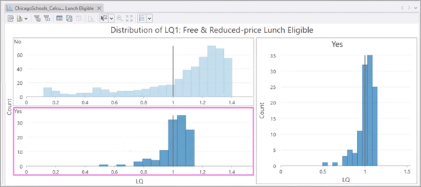
- Distribution of Location Quotients—A histogram of the location quotients. Use the chart to identify extreme values and observe the shape of the distribution. If the Benchmark Type parameter value is Stratified (case-field) the chart will include a histogram for each unique case.
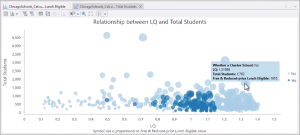
- Relationship between the Location Quotient and Total Variable- A scatter plot showing the relationship between the total variable and the location quotient for each feature. The size of the points is proportional to the analysis variable, so bigger points reflect features with larger analysis variable values. If the Benchmark Type parameter value is Global (all features) or Reference rate, color symbolizes the location quotient and matches the layer's color ramp. If the Benchmark Type parameter value is Stratified (case-field), each color represents a unique case-field.
Note:
Large location quotients with a small total variable value may not be stable. The large location quotient may reflect the small total variable.
Pop-up charts
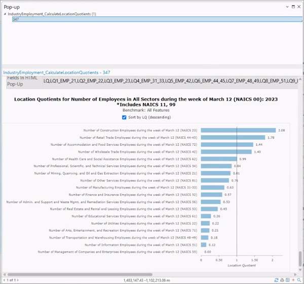
Pop-up charts are generated for each output feature and can be viewed by clicking on the feature in the map. The bar chart displays the location quotient. If you calculate multiple location quotients, the bar chart will include a bar for each analysis variable. Location quotients are displayed on the x-axis; the location quotient value for each analysis variable also appears as text at the end of each bar. The chart includes a guideline where location quotient is equal to 1. Use the Sort by LQ (descending) checkbox to sort the location quotients in descending order.
References
Cromley, Robert G. and Hanink, Dean M. 2012. “Focal Location Quotients.” Geographical Analysis. Vol. 44: 398-410. https://doi.org/10.1111/j.1538-4632.2012.00852.x
Isserman, A. M. (1977). The Location Quotient Approach to Estimating Regional Economic Impacts. Journal of the American Institute of Planners, 43(1), 33–41. https://doi.org/10.1080/01944367708977758
Miller, M. M., Gibson, L. J., & Wright, N. G. (1991). Location Quotient: A Basic Tool for Economic Development Analysis - ProQuest (Pt. 65). Economic Development Review, 9(2). https://www.proquest.com/openview/d6011b83d027b7ad1dba29bb96b74a53/1?pq-origsite=gscholar&cbl=38209