Spatial Autoregression (Spatial Statistics Tools)
Summary
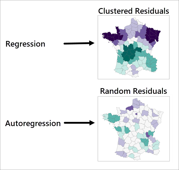
Estimates a global spatial regression model for a point or polygon feature class.
The assumptions of traditional linear regression models are often violated when using spatial data. When spatial autocorrelation is present in a dataset, coefficient estimates may be biased and lead to overconfident inference. This tool can be used to estimate a regression model that is robust in the presence of spatial dependence and heteroskedasticity, as well as measure spatial spillovers. The tool uses Lagrange Multiplier (LM), also known as a Rao Score, diagnostic tests to determine the model that is most appropriate. Based on the LM diagnostics, either an ordinary least square (OLS), spatial lag model (SLM), spatial error model (SEM), or spatial autoregressive combined model (SAC) may be estimated.
Illustration
Usage
The tool accepts only point and polygon inputs.
The dependent variable must be continuous (not binary or categorical).
Explanatory variables must be continuous (not binary or categorical). Do no use binary variables (containing only the values 0 and 1, as they may violate model assumptions and cause an error.
The output of the tool includes a Moran's Scatter Plot of Residuals that can be used to identify autocorrelation in the model's residuals.
The spatial weights matrix used cannot have more than 30 percent connectivity. An error will occur if this threshold is reached to prevent biased estimates.
When using k nearest neighbors with a local weighting scheme, an adaptive bandwidth will be calculated if no bandwidth is provided.
A Spatial Durbin model can be estimated by fitting a SLM and including each explanatory variable and their spatial lags. Use the Neighborhood Summary Statistics tool to calculate spatial lags.
The models are estimated using the following methods related to heteroskedasticity and normality:
SLM uses Spatial Two Stage Least Squares regression (S2SLS).
SEM uses Generalized Method of Moments (GMM).
SAC uses Generalized S2SLS (GS2SLS).
Parameters
| Label | Explanation | Data type |
|---|---|---|
|
Input Features |
The input features containing the dependent and explanatory variables. |
Feature Layer |
|
Dependent Variable |
The numeric field that will be predicted in the regression model. |
Field |
|
Explanatory Variables |
A list of fields that will be used to predict the dependent variable in the regression model. |
Field |
|
Output Features |
The output feature class containing the predicted values of the dependent variable and the residuals. |
Feature Class |
|
Model Type |
The model type that will be used for the estimation. By default, LM diagnostic tests will be used to determine the model that is the most appropriate for the input data.
|
String |
|
Neighborhood Type (Optional) |
Specifies how neighbors will be chosen for each input feature. To identify local spatial patterns, neighboring features must be identified for each input feature.
|
String |
|
Distance Band (Optional) |
The distance within which features will be included as neighbors. If no value is provided, one will be estimated during processing and included as a geoprocessing message. |
Linear Unit |
|
Number of Neighbors (Optional) |
The number of neighbors that will be included as neighbors. The number does not include the focal feature. The default is 8. |
Long |
|
Weights Matrix File (Optional) |
The path and file name of the spatial weights matrix file that defines spatial relationships among features. |
File |
|
Local Weighting Scheme (Optional) |
Specifies the weighting scheme that will be applied to neighbors. Weights will always be row-standardized unless a spatial weights matrix file is provided.
|
String |
|
Kernel Bandwidth (Optional) |
The bandwidth of the weighting kernel. If no value is provided, an adaptive kernel will be used. An adaptive kernel uses the maximum distance from a neighbor to a focal feature as the bandwidth. |
Linear Unit |
Environments
Licensing information
- Basic: Yes
- Standard: Yes
- Advanced: Yes