Summary statistics
Summary statistics are calculated by the Aggregate Points, Summarize Within, Summarize Nearby, Join Features, and Dissolve Boundaries tools.
Equations
Mean and standard deviation are calculated using weighted mean and weighted standard deviation for line and polygon features. None of the statistics for point features are weighted. The weight is the length or area of the feature that falls within the boundary.
The following table shows the equations used to calculate standard deviation, weighted mean, and weighted standard deviation:
|
Statistic |
Equation |
Variables |
Features |
|---|---|---|---|
|
Standard Deviation |
\(\displaystyle sd=\sqrt{\frac{1}{N-1}\sum_{i=1}^{N}(x_i-x̄)²}\) |
where:
|
Points |
|
Weighted Mean |
\(\displaystyle x̄_w=\frac{\sum_{i=1}^{N}(w_i*x_i)}{\sum_{i=1}^{N}w_i}\) |
where:
|
Lines and polygons |
|
Weighted Standard Deviation |
\(\displaystyle sd_w=\sqrt{\frac{\sum_{i=1}^{N}w_i(x_i-x̄_w)²}{\frac{(N'-1)}{N'}\sum_{i=1}^{N}w_i}}\) |
where:
|
Lines and polygons |
Note:
Null values are excluded from all statistical calculations. For example, the mean of 10, 5, and a null value is:
\(\displaystyle \frac{10+5}{2}=7.5\)
Points
Point layers are summarized using only the point features within the boundary areas.
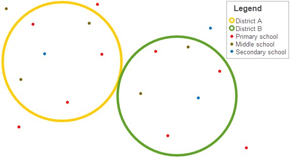
A real-life scenario in which points could be summarized is in determining the total number of students in each school district. Each point represents a school. The Type field gives the type of school (primary school, middle school, or secondary school) and a population field gives the number of students enrolled at each school.
The figure below shows a hypothetical point and boundary layer, and the table summarizes the attributes for the point layer.
| ObjectID | District | Type | Population |
|---|---|---|---|
| 1 | A | Primary school | 280 |
| 2 | A | Primary school | 408 |
| 3 | A | Primary school | 356 |
| 4 | A | Middle school | 361 |
| 5 | A | Middle school | 450 |
| 6 | A | Secondary school | 713 |
| 7 | B | Primary school | 370 |
| 8 | B | Primary school | 422 |
| 9 | B | Primary school | 495 |
| 10 | B | Middle school | 607 |
| 11 | B | Middle school | 574 |
| 12 | B | Secondary school | 932 |
The calculations and results for District A are given in the table below. From the results, you can see that District A has 2,568 students. When running a tool, the results would also be given for District B.
|
Statistic |
Result District A |
|---|---|
|
Sum |
\(280+408+356+361+450+713=2568\) |
|
Minimum |
Minimum of: \(\left[\begin{array}{cccc}280, & 408, & 356, \\361, & 450, & 713\end{array}\right] = 280\) |
|
Maximum |
Maximum of: \(\left[\begin{array}{cccc}280, & 408, & 356, \\361, & 450, & 713\end{array}\right] = 713\) |
|
Mean |
\(\displaystyle \frac{2568}{6}=428\) |
|
Standard Deviation |
\(\displaystyle \sqrt{\frac{(280-428)²+(408-428)²+(356-428)²+(361-428)²+(450-428)²+(713-428)²}{6-1}}\) \(=150.79\) |
Lines
Line layers are summarized using only the proportions of the line features that are within the boundary areas.
Tip:
When summarizing lines, use fields with counts or amounts so proportional calculations make logical sense in your analysis. For example, use population rather than population density.
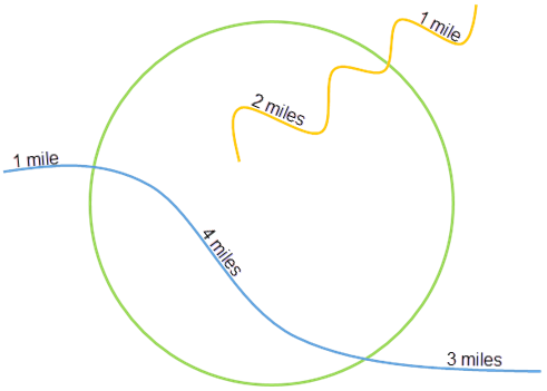
A real-life scenario in which you can use this analysis is determining the total volume of water in rivers within a specified boundary. Each line represents a river that is partially located inside the boundary.
The figure below shows a hypothetical line and boundary layer, and the table summarizes the attributes for the line layer.
| River | Length (miles) | Volume (gallons) |
|---|---|---|
| Yellow | 3 | 6,000 |
| Blue | 8 | 10,000 |
The calculations for volume are given in the table below. From the results, you can see that the total volume is 9,000 gallons.
Note:
The calculations use the proportions of the lines within the boundary area. For example, the yellow line has a total volume of 6,000 gallons with two of its three total miles within the boundary. Therefore, the calculations are preformed using 4,000 gallons as the volume for the yellow line:
\(\displaystyle \frac{6000 * 2}{3}=4000\)
|
Statistic |
Result |
|---|---|
|
Sum |
\(4000+5000=9000\) |
|
Minimum |
Minimum of: \(\left[\begin{array}{cc}4000, & 5000\end{array}\right] = 4000\) |
|
Maximum |
Maximum of: \(\left[\begin{array}{cc}4000, & 5000\end{array}\right] = 5000\) |
|
Mean |
\(\displaystyle \frac{(2 * 4000)+(3 * 5000)}{2+3} = 4600\) |
|
Standard Deviation |
\(\displaystyle \sqrt{\frac{2(4000-4600)²+3(5000-4600)²}{\frac{2-1}{2}(2+3)}} = 692.8\) |
Polygons
Polygon layers are summarized using only the proportions of the polygon features that are within the boundary areas.
Tip:
When summarizing polygons, use fields with counts or amounts so proportional calculations make logical sense in your analysis. For example, use population rather than population density.
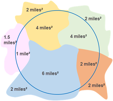
A real-life scenario in which you can use this analysis is determining the population in a city neighborhood. The blue outline represents the boundary of the neighborhood and the smaller polygons represent census blocks.
The figure below shows a hypothetical polygon and boundary layer, and the table summarizes the attributes for the polygon layer.
| Census block | Area (miles²) | Population |
|---|---|---|
| Yellow | 6 | 3,200 |
| Green | 6 | 4,700 |
| Pink | 2.5 | 1,000 |
| Blue | 8 | 4,500 |
| Orange | 4 | 3,600 |
The calculations for population are given in the table below. From the results, you can see that there are 10,841 people in the neighborhood and an average (mean) of approximately 2,666 people per census block.
Note:
The calculations use the proportions of the polygons within the boundary area. For example, the yellow polygon has a total population of 3,200 with four of its six total square miles within the boundary. Therefore, the calculations are preformed using 2,133 as the population for the yellow polygon:
\(\displaystyle \frac{3200 * 4}{6}=2133\)
|
Statistic |
Result |
|---|---|
|
Sum |
\(2133+3133+400+3375+1800=10841\) |
|
Minimum |
Minimum of: \(\left[\begin{array}{ccc}2133, & 3133, & 400, \\3375, & 1800\end{array}\right] = 400\) |
|
Maximum |
Maximum of: \(\left[\begin{array}{ccc}2133, & 3133, & 400, \\3375, & 1800\end{array}\right] = 3375\) |
|
Mean |
\(\displaystyle \frac{(4 * 2133)+(4 * 3133)+(1 * 400)+(6 * 3375)+(2*1800)}{4+4+1+6+2} = 2665.53\) |
|
Standard Deviation |
\(\displaystyle \sqrt{\frac{4(2133-2665.53)²+4(3133-2665.53)²+1(400-2665.53)²+6(3375-2665.53)²+2(1800-2665.53)²}{\frac{5-1}{5}(4+4+1+6+2)}}\) \(= 925.91\) |
Related topics
Use the following topics to learn more about summary statistics within a specific tool: