Tutorial: Create satellite imagery products using ArcGIS Pro Ortho mapping

Available with Advanced license.

In ArcGIS Pro, you can photogrammetrically correct satellite imagery to remove geometric distortions induced by the platform and terrain displacement. After removing these distortions, you can generate ortho mapping products, including orthomosaic, digital surface model (DSM) and a DSM mesh. In this tutorial, you will generate a high-resolution DSM and orthomosaic.

First, you will set up an ortho mapping workspace to manage your satellite imagery collection. Next, you will perform a block adjustment, followed by a refined adjustment using ground control points. Finally, you'll generate an orthorectified mosaic (orthomosaic) and DSM.

ArcGIS Pro can process satellite images from many sensor platforms, as long as the image orientation is described by a rational polynomial coefficients (RPC) model or a rigorous sensor model. This model is typically imbedded in the image file or included as a separate metadata file.

Create an ortho mapping workspace

An ortho mapping workspace is an ArcGIS Pro subproject that is dedicated to ortho mapping workflows. It is a container within an ArcGIS Pro project folder that stores the resources and derived files that belong to a single image collection in an ortho mapping task.

The imagery packaged for this tutorial was collected and provided by Maxar Technologies. It includes a pair of multispectral and panchromatic images, a table of ground control points, and a DEM.

To create an ortho mapping workspace, complete the following steps:

1. Download the tutorial dataset, unzip it and save the content to C:\SampleData\orthomapping_satellite_tutorial.

2. In ArcGIS Pro, create a project using the Map template.

3. On the Imagery tab, in the Ortho Mapping group, click the New Workspace drop-down menu and select New Workspace.

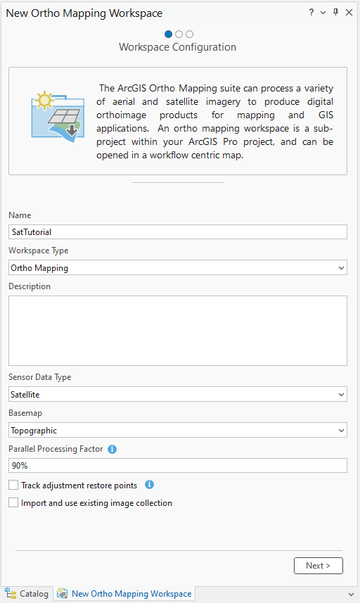
4. In the Workspace Configuration window, type a name for your workspace.

5. In the Type drop-down menu, choose Satellite.

6. Optionally, from the Basemap drop-down list, choose a basemap as a backdrop for the image collection.

7. Set the Parallel Processing Factor value of the workspace to 90%.

   Setting the Parallel Processing Factor value to 90% means that 90% of total CPU cores will be used to support Ortho mapping processing. The Parallel Processing Factor value can also be changed in Properties in the Workspace group in the Imagery tab after the workspace is created.

   Setting the Parallel Processing Factor value higher than what your system can accommodate will lead to parallel processing failures. A common requirement is that for each logical processor, you need 2GB of RAM. For example, if you are working with a system that has 6 cores, 12 logical processors, and 16 GB RAM, setting the parallel processing factor to 100 percent would require a minimum 24 GB of RAM for the process to run successfully. A more appropriate Parallel Processing Factor value based on this example would be 50 percent. which would require approximately 12 GB of RAM.

8. Click Next.

   

9. In the Image Collection window, for Sensor Type, choose GeoEye-1.

10. Under Folder Containing Images, click the Browse button and navigate to the tutorial data folder on your machine and select the imagery folder (GeoEye_NAD83_UTM10N), then click OK.

    The appropriate Workspace Spatial Reference information is automatically populated.

    

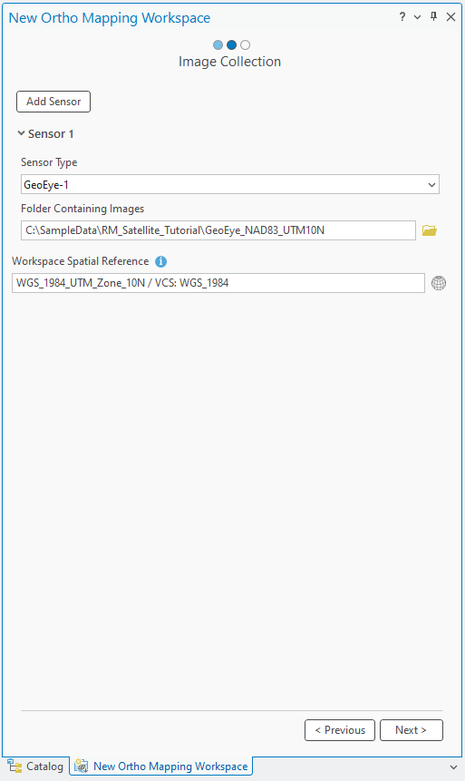
11. Click Next.

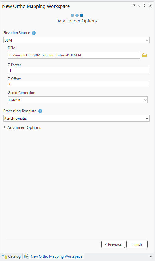
12. In the Data Loader window, under Elevation Source, choose DEM. Under DEM, browse to the DEM provided with the tutorial dataset.

    Note:

    This DEM will be used to support the block adjustment process.

13. Most elevation data uses orthometric heights, so you will need to apply a geoid correction. Under Geoid correction, ensure EGM96 is selected.

14. Under Processing Template, choose Panchromatic.

15. Expand Advanced Options.

16. Ensure Estimate Statistics option is checked.

17. Accept all other defaults and click Finish.

    

    Once the workspace has been created, the images and image footprints will be displayed in the map. A Ortho Mapping category has also been added to the Contents pane, where the source imagery data and derived Ortho mapping products will be stored.

    The initial display of imagery in the workspace confirms that all images and necessary metadata were provided to initiate the workspace. The images have not been aligned or adjusted, so the mosaic may not appear geometrically correct.

    A new Ortho Mapping tab will be added to the ArcGIS Pro main menu. Clicking this tab will expose a series of tools and workflows dedicated to Ortho mapping. In the Product category, all the buttons are unavailable because the images are not yet adjusted.

    

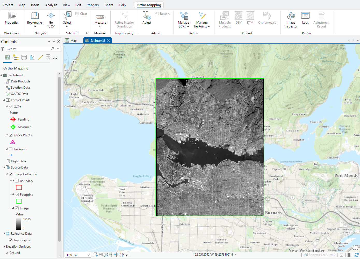
    Satellite image © 2020 Maxar Technologies

Perform a block adjustment

After creating ortho mapping workspace, the next step is to perform block adjustment using the tools in the Adjust and Refine groups. The block adjustment will first calculate tie points, which are common points in areas of image overlap. The tie points will then be used to calculate the orientation of each image, known as "exterior orientation" in photogrammetry.

1. On the Ortho Mapping tab, in the Adjust group, click Adjust .

2. In the Adjust window, under Transformation Type, choose RPC. The Rational Polynomial Coefficients (RPC) transformation will be applied in the adjustment, which is used for satellite imagery that contains RPC information within the metadata.

3. Check the box next to Reproject Tie Points.

   This will ensure that the tie point map coordinates are calculated.

4. Expand the Tie Point Matching section and ensure your parameter settings match those in the example below.

   

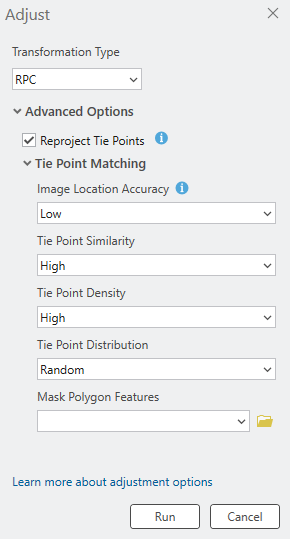
5. Click Run to perform block adjustment.

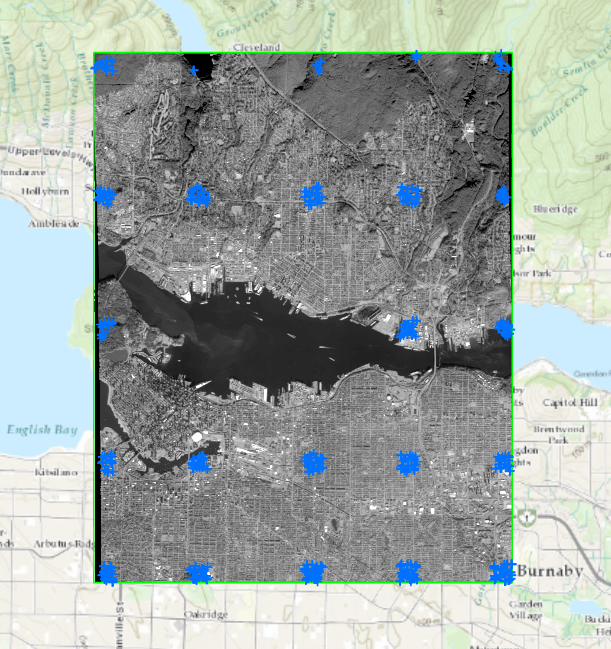
6. After the adjustment is complete, turn on the Tie Points layer in the Contents pane to view the distribution of generated tie points on the map. Your tie point distribution may differ from that shown below.

   

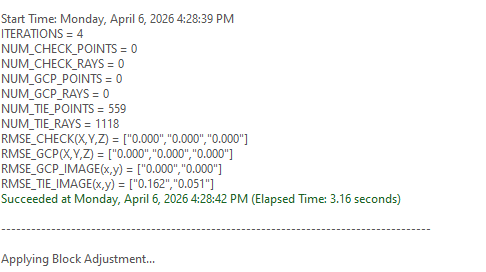
7. Tie point residuals or accuracy reporting can be viewed in the logs file. On the Ortho Mapping tab, in the Review group, click Logs to access Logs file. Tie point residuals are displayed in the row labeled RMSE_Tie_Image(x,y). The units for tie point RSME is pixels.

   Your residual may differ slightly from the example below.

   

Following the initial adjustment, notice that all buttons in the Product category are now active. These buttons highlight the imagery products that can be generated. Before generating products, ground control points will be used to improve the absolute accuracy of the images.

Add Ground Control Points (GCP)

Ground control points (GCPs) are points with known x,y,z ground coordinates. They are often obtained from ground survey or existing data and used to ensure that the images will be accurately georeferenced in the ground coordinate system. Block adjustment can be applied without GCPs and still ensure relative accuracy, but adding GCPs increases the absolute accuracy of the adjusted imagery. If you do not have GCPs from a ground survey, but you have a georeferenced raster layer (raster dataset, mosaic dataset, or image service), you can add it as a reference to compute GCPs.

GCPs selected from a reference layer and saved in a text file can also be imported and used to enhance adjustment accuracy. For this tutorial, you'll use this import method to add GCPs to the project.

To import GCPs, complete the following steps:

1. On the Ortho Mapping tab, in the Refine group, click Manage GCPs to open the GCP Manager.

2. In the GCP Manager window, click the Import GCPs button .

3. In the Import GCPs window, browse to and select the GCP file (Vancouver_NAD83-UTM10N.csv). Click OK.

4. Under Set GCP Spatial Reference, click the Browse button . For Horizontal systems, expand Projected Coordinate System, North America, Zone Series, and UTM (NAD 1983), and choose NAD 1983 UTM Zone 10N. Click OK to accept the changes and close the Spatial Reference window.

   The vertical coordinate system (VCS) was not set because the digital elevation model used to extract height values for the GCPs did not have a VCS defined. If the DEM you used had a defined VCS, the vertical systems would have been set with matching coordinates.

5. For Geographic Transformations, click the Horizontal tab and choose WGS 1984 (ITRF00) To NAD 1983 from the drop-down list.

6. Ensure the field mappings are correct.

7. Click the browse button below GCP Photo Location and browse to and select the folder containing the images of the GCP locations. Click OK.

8. For Photo File Extension, choose PNG from the drop-down list.

   

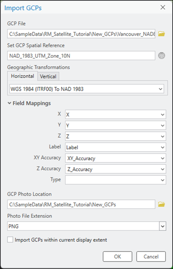
9. Click OK to import the GCPs.

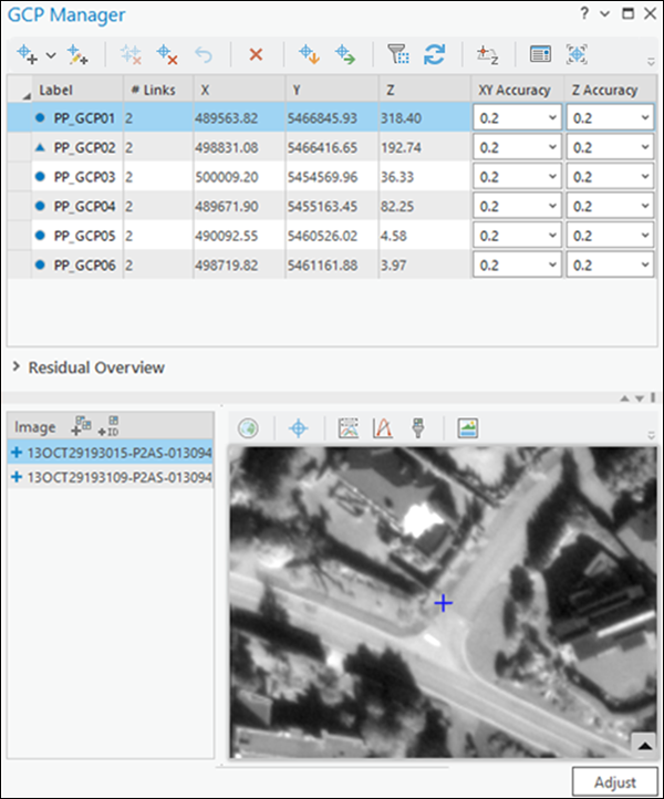
   Once the GCPs have been imported, the table in the GCP Manager will be populated.

   

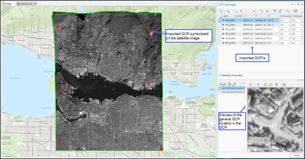
   In GCP Manager, the first GCP in the list will be selected by default, and a preview of the image where the GCP is located is displayed in the Preview section.

10. To add tie points for the selected GCP, in the Preview section, click the View GCP Photo button to display the GCP image chip. Use the mouse wheel to zoom in on the image chip to see the GCP location indicated by a red arrow.

11. Click the drop down next to the Add GCP or Tie Point button in the GCP Manager window and select Semi-Auto to add a tie point in the image viewer for each image.

    The tie points for other images will be automatically calculated by the image matching algorithm where possible, although each tie point should be checked for accuracy. If the tie point is not automatically identified, add the tie point manually by selecting the appropriate location in the image.

12. Repeat steps 10 and 11 to select and add tie points for the remaining GCPs.

13. After each GCP has been measured with tie points, select point PP_GCP02 and right-click to change it to a Check Point. This point will be excluded in the adjustment process and will instead be used to independently assess the accuracy of the adjustment results.

14. After adding GCPs and checkpoints, the adjustment must be run again to incorporate these points. Click Adjust.

    

Review Adjustment Results

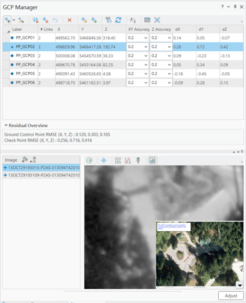
Adjustment quality results can be viewed in GCP Manager by analyzing the residuals for each GCP. Residuals represent the difference between the measured and computed position of a point. They are measured in the units of the project spatial referencing system. After completing adjustment with GCPs, three new fields, dX, dY, and dZ, are added to the GCP Manager table and display the residuals for each GCP. The quality of the fit between the adjusted block and the map coordinate system can be evaluated using these values. The Root Mean Square Error (RMSE) of the residuals can be viewed by expanding the Residual Overview section of GCP Manager.

Additional adjustment statistics are provided in the adjustment report. To generate the report, under the Ortho Mapping tab, in the Review group, click Adjustment Report.

Generate a Digital Surface Model (DSM)

Once the block adjustment is complete, 2D imagery products can be generated using the tools in the Product group on the Reality Mapping tab. The stereo image pairs of an image collection are used to generate a point cloud (3D points) for which elevation data can be derived. The derived elevation data is classified as either a digital terrain model (DTM), which includes only the ground surface, or a digital surface model (DSM), which includes the elevations of trees, buildings, and other above ground features.

Note:

If an area is heavily wooded, or has other dense vegetation cover, it will not be possible to derive a DTM ground surface because the ground is not visible. This issue might also arise in a dense urban areas, where buildings obscure the ground. In this case, the most appropriate elevation surface is a DSM, which specifically creates a surface depicting the top of the urban environment.

Follow the steps below to generate a DSM using the wizard.

1. On the Ortho Mapping tab, click the DSM button in the Product group.

   The Ortho Mapping Products Wizard window appears.

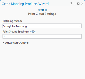
2. Click Next to advance the wizard to the Point Cloud Settings window.

3. In the Point Cloud Settings window, for Matching Method, choose Semiglobal Matching from the drop-down menu.

   This method is typically used for images of urban areas and captures more detailed terrain information.

4. Accept the default Point Ground Spacing value.

   This defines the spacing, in meters, at which the 3D points are generated. The default is three times the resolution of the source imagery.

5. Accept all remaining default settings and click Next.

   For information on Advanced Settings, see Create elevation data using the ortho mapping DEMs wizard.

   

6. In the DSM Settings window, for Cell Size, use the default value of 3 x GSD.

   This will determine the resolution of the DSM, which is three times the imagery resolution, in this case.

7. Accept the remaining default settings and click Finish.

   The DSM will be generated.

Generate a orthomosaic

Next, you will generate an orthomosaic. An orthomosaic is an orthorectified image product mosaicked from an image collection. Geometric distortion has been corrected and the imagery has been color balanced to produce a mosaic.

1. On the Ortho Mapping tab, in the Product group, click Orthomosaic to start the Orthomosaic Wizard.

2. Ensure Color Balance and Generate Seamlines options are checked.

3. Click Next.

4. In the Color Balance Settings pane, for Balance Method, select Dodging from the drop-down list and accept all other default options.

5. Click Next.

6. In the Seamline Settings window, for Computation Method, select Voronoi in the drop-down list.

7. Expand the Processing section, and input 20 for Blend Width.

   

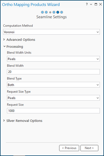
8. Click Next.

   The wizard guided workflow advances to the next pane, Orthomosaic Settings.

9. Accept all the default settings in the Orthomosaic Settings pane, and click Finish.

   The orthomosaic will be generated, listed in the Contents pane, and loaded into the map display.

   Note:

   Multiple products can be generated simultaneously using the Multiple Products wizard.

Summary

In this tutorial, you created an ortho mapping workspace for satellite imagery and used tools on the Ortho Mapping tab to apply a photogrammetric adjustment with ground control points. You then used the Ortho Mapping DSM wizard to generate a DEM and an orthomosaic..

The satellite imagery used in this tutorial was acquired and provided by Maxar Technologies.

Related topics

• Ortho mapping in ArcGIS Pro

• Tutorial: Create drone imagery products using ArcGIS Pro Ortho Mapping

• Tutorial: Create digital aerial imagery products with ArcGIS Pro Ortho Mapping