Tutorial: Create drone imagery products with ArcGIS Pro Ortho mapping using Server
![]() Available with Advanced license.
Available with Advanced license.
In ArcGIS Pro, you can use photogrammetry to correct drone imagery to remove geometric distortions caused by the sensor, platform, and terrain displacement. After removing these distortions, you can generate Ortho mapping products. This processing can be performed remotely on your self-hosted enterprise infrastructure, enabling you to leverage multi-machine configuration for distributed processing.
First, you will set up an Ortho mapping workspace to manage the drone imagery collection using the New Ortho Mapping Workspace wizard. Next, you will perform a block adjustment, followed by a refined adjustment using ground control points. Finally, you'll generate a digital surface model (DSM), and an orthorectified mosaic, or orthomosaic, using the Ortho Mapping Products Wizard.
Ortho mapping requires information about the camera, including focal length and sensor size, as well as the location at which each image was captured. This information is commonly stored as metadata in the image files, typically in the EXIF header. It is also helpful to know the GPS accuracy. In the case of drone imagery, this should be provided by the drone manufacturer. The GPS accuracy for the sample dataset in this tutorial is better than 5 meters.
Note:
ArcGIS Image Server configured for raster analysis or ArcGIS Reality Server is needed to complete this tutorial. To set up an ArcGIS Image Server raster analysis site, please see raster analytics deployment. For Reality Server configuration, please refer to the Reality Server installation.
Connect to Server
To utilize Server for processing your data in ArcGIS Pro, you need to first connect to the Server.
Open ArcGIS Pro, Click the Project tab on the ribbon and click the Portals page.
You can also access the portals page from the Manage Portals link in the Sign In menu
 .
.Click Add Portal.
Enter the URL (
https://webadaptorhost.domain.com/webadaptorname) for the portal on the Add Portal dialog box and click OK.Sign in to the portal by clicking the Options button
 or right-click the portal and click Sign in. Enter your username and password.
To make the new connection your active portal, right-click the URL and click Set As Active Portal.
Once you successfully connect to your portal, your username will show up in the top right corner of ArcGIS Pro.
Create an Ortho mapping workspace
An Ortho mapping workspace is an ArcGIS Pro subproject that is dedicated to Ortho mapping workflows. It is a container in an ArcGIS Pro project folder that stores the resources and derived files that belong to a single image collection in an Ortho mapping task.
A collection of 195 drone images is provided for this tutorial. The GCP folder contains the Tut_Ground_Control_UTM11N_EGM96.csv file, which contains ground control points (GCPs), and a file geodatabase (GCP_desc.gdb) with a Ground_Control_NAD832011_NAVD88 point feature class identifying the GCP locations at the site.
To create an ortho mapping workspace, complete the following steps:
Download the tutorial dataset. unzip it, and save contents to
C:\SampleData\RM_Drone_tutorial.In ArcGIS Pro, create a project using the Map template.
On the Imagery tab, in the Reality Mapping group, click the New Workspace drop-down menu and choose New Workspace.
In the Workspace Configuration window, type a name for the workspace.
Click the Workspace Type drop-down list, and choose Ortho Mapping.
Ensure that the Sensor Data Type is set to Drone.
Click the Basemap drop-down menu, and choose Topographic.
Set the Parallel Processing Factor. This controls the maximum computational resource for distributed processing. It is recommended to use percentage expression. For example, if you have 2 Server nodes, set Parallel Processing Factor to 50% to utilize one machine for block adjustment and ortho mapping product generation.
Check Process this image collection on server.
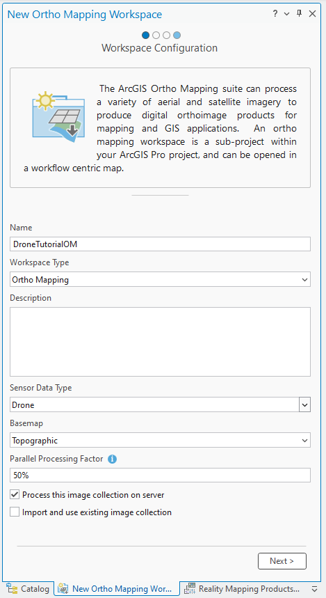
Accept all other default values and click Next.
The Image Collection window appears.
In the Image Collection window, for Sensor Type, ensure that Generic is chosen.
This option is used because the imagery was collected with an RGB camera.
Click Source, ensure File is selected from the drop-down list.
Click Add, browse to the tutorial data location, select the Images folder, then click OK.
Note:
Most modern drones store GPS information in the EXIF header. This will be used to automatically populate the table shown below. However, some older systems or custom-built drones may store GPS data in an external file. In this case, you can use the Import button
 next to the Geolocation parameter to import external GPS files.
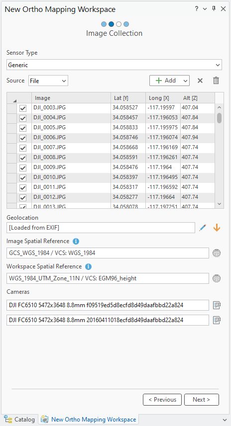
The Spatial Reference and Camera Model values are automatically populated. The workspace requires a projected coordinate system. The autogenerated, default Workspace Spatial Reference is based on the matching WGS84 UTM coordinates for the images. This projection determines the spatial reference for your ortho products, including the orthomosaic and DEM.
Click Next.
In the Data Loader Options page, for Elevation Source, select Average Elevation from DEM from the drop-down list. The World Elevation Service will be used as the Elevation Source.
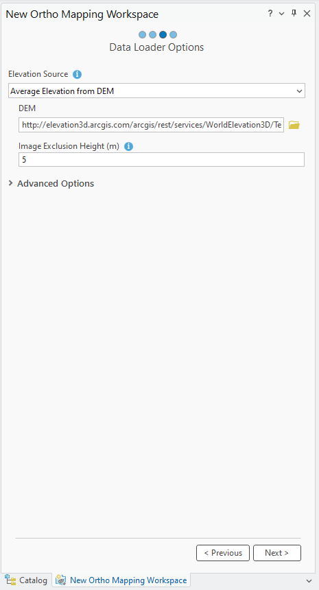
If you have access to the internet, the Elevation Source value is derived from the World Elevation Service. This provides an initial estimate of the flight height for each image.
If you do not have access to the internet or a DEM, choose Constant Elevation from the Elevation Source drop-down menu and enter an elevation value of 414 meters.
The parameter, Image exclusion Height (m), refers to the image exclusion height, where images having a flight height above terrain that is less than this value will not be included in the workspace.
Accept other default settings in the Data Loader Options window and click Next.
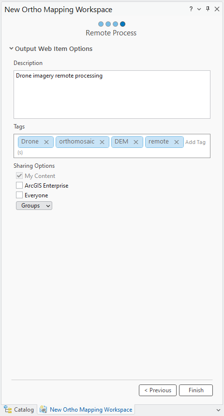
In the Remote Process window, provide description and tags for the image service and click Finish.
Once the workspace has been created, the images and drone path are displayed. An Ortho Mapping category is added to the Contents pane, where the image collection image service and derived Ortho mapping products service will be stored.
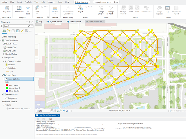
To see the image footprints, you can right click on the Image Collection in the Contents pane > Properties > Display > Check on Display Footprints.
The initial display of imagery in the workspace confirms that all images and necessary metadata were provided to initiate the workspace. The images have not been aligned or adjusted, so the mosaic may not appear geometrically correct. Note: You may need to zoom in close enough to see the image.
A new Ortho Mapping tab will be added to the ArcGIS Pro main menu. Clicking this tab will expose a series of tools and workflows dedicated to Ortho mapping. In the Product category, all the buttons are unavailable because the images are not yet adjusted.
Perform a block adjustment
After the Ortho mapping workspace has been created, the next step is to perform a block adjustment using the tools in the Adjust and Refine groups. The block adjustment first calculates tie points, which are common points in areas of image overlap. The tie points are then used to calculate the orientation of each image, known as exterior orientation in photogrammetry. The block adjustment process may take a few hours depending on your computer setup and resources.
To perform a block adjustment, complete the following steps:
On the Ortho Mapping tab, in the Adjust group, click Adjust
 .
.In the Adjust window, ensure all the Perform Camera Calibration options are checked.
This indicates that the input focal length is approximate and that the lens distortion parameters will be calculated during adjustment. For drone imagery, these options are checked by default, since most drone cameras have not been calibrated. This option should not be checked for high-quality cameras with known calibration. The camera self-calibration requires that an image collection has in-strip overlap of more than 60 percent and cross-strip overlap of more than 30 percent.
Expand Advanced Options.
Ensure Use Orientations from Metadata option is checked.
This reduces the adjustment duration by using the exterior orientation information embedded in the image EXIF as initial values.
Ensure the Fix Image Location for High Accuracy GPS option is unchecked.
This option is used only for imagery acquired with differential GPS, such as Real Time Kinematic (RTK) or Post Processing Kinematic (PPK).
Optionally, uncheck Compute Posterior Standard Deviation for Images.
For Image Location Accuracy, choose High from the drop-down menu.
GPS location accuracy indicates the accuracy level of the GPS data collected concurrently with the imagery and listed in the corresponding EXIF data file. This is used in the tie point calculation algorithm to determine the number of images in the neighborhood to use. The High value is used for GPS accuracy from 0 to 10 meters.
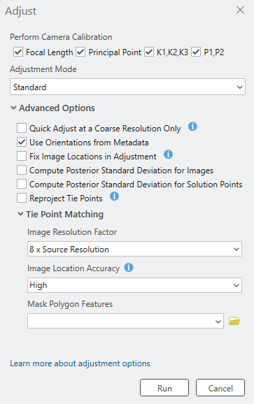
Accept all other defaults and click Run.
After the adjustment has been performed, the
Logsfile displays statistical information such as the mean reprojection error (in pixels), which signifies the accuracy of adjustment, the number of images processed, and the number of tie points generated.The relative accuracy of the images is also improved, and derived products can be generated using the options in the Product category. To improve the absolute accuracy of generated products, GCPs must be added to the block.
Add GCPs
GCPs are points with known x,y,z ground coordinates, which are often obtained from ground survey, that are used to ensure that the photogrammetric process has reference points on the ground. A block adjustment can be applied without GCPs and still ensure relative accuracy, although adding GCPs increases the absolute accuracy of the adjusted imagery.
Import GCPs
To import GCPs, complete the following steps:
On the Ortho Mapping tab, in the Refine group, click Manage GCPs.
The GCP Manager window appears.
In the GCP Manager window, click the Import GCPs button
 .
.In the Import GCPs window, under GCP File, browse to and select the
Tut_Ground_Control_UTM11N_EGM96.csvfile, and click OK.Under Set GCP Spatial Reference, click the Spatial Reference button
 and do the following in the Spatial Reference window:
For Horizontal systems, expand Projected Coordinate System, North America, Zone Series, and UTM (NAD 1983), and choose NAD 1983 UTM Zone 11N.
To define the vertical coordinate system, click the vertical systems tab, expand Vertical Coordinate System, Gravity-related, and World, and choose EGM96 height.
Click OK to accept the changes and close the Spatial Reference window.
Under Geographic Transformations, click the Horizontal tab and choose WGS 1984 (ITRF00) to NAD83 from the drop-down list.
Click the Vertical tab and choose None from the drop-down menu.
Map the GCP fields accordingly under Field Mappings.
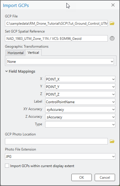
Click OK to import the GCPs.
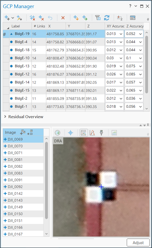
The imported GCPs are listed in the GCP Manager window, and the relative locations are displayed in the 2D Map view with a red position indicator
 .
.Click the drop down next to the Add GCP or Tie Point button in the GCP Manager window and select Semi-Auto
 .
.Click one of the GCPs in the table of the GCP Manager window. A list of images containing the GCP will be displayed in the lower panel of the GCP manager window.
Click on one of the listed images and select the exact location of the GCP in the image viewer to add a tie point.
Using the Semi_Auto GCP option, the tie points for other images are automatically calculated by the image matching algorithm, when possible, indicated by a blue cross next to the image ID. Review each tie point for accuracy. If the tie point is not automatically identified, add the tie point manually by selecting the appropriate location in the image.
Repeat step 11 and 12 for the other GCPs.
After each GCP has been added and measured with tie points, select one of the GCPs, right-click, and change it to a check point.
This provides a measure of the absolute accuracy of the adjustment, as check points are not used in the adjustment process.
After adding GCPs and check points, click Adjust to run the adjustment again to incorporate these points.
Review adjustment results
Adjustment quality results can be viewed in the GCP Manager window by analyzing the residuals for each GCP. Residuals represents the difference between the measured position and the computed position of a point. They are measured in the units of the project's spatial referencing system. After completing adjustment with GCPs, three new fields—dX, dY, and dZ—are added to the GCP Manager table and display the residuals for each GCP. The quality of the fit between the adjusted block and the map coordinate system can be evaluated using these values. The root mean square error (RMSE) of the residuals can be viewed by expanding the Residual Overview section of the GCP Manager window.
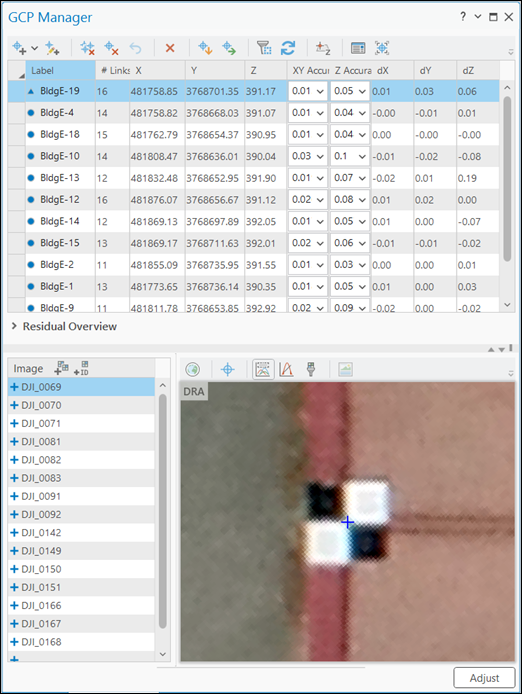
Additional adjustment statistics are provided in the adjustment report. To generate the report, on the Ortho Mapping tab, in the Review group, click Adjustment Report.
Generate a DSM
The stereo image pairs of an image collection are used to generate a point cloud (3D points) for which elevation data can be derived. The derived elevation data is classified as either a digital terrain model (DTM), which includes only the ground surface, or a digital surface model (DSM), which includes the elevations of trees, buildings, and other above ground features.
Note:
Elevation values can be derived when the image collection has a good amount of overlap to form the stereo pairs. Typical image overlap necessary to produce point clouds is 80 percent forward overlap along a flight line and 60 percent overlap between flight lines.
Follow the steps below to generate a DSM using the wizard.
On the Ortho Mapping tab, click the DSM button
 in the Product group.
The Ortho Mapping Products Wizard window appears.
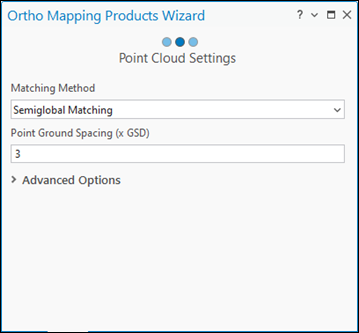
Click Next to advance the wizard to the Point Cloud Settings window.
In the Point Cloud Settings window, for Matching Method, choose Semiglobal Matching from the drop-down menu.
This method is typically used for images of urban areas and captures more detailed terrain information.
Accept the default Point Ground Spacing value.
This defines the spacing, in meters, at which the 3D points are generated. The default is three times the resolution of the source imagery.
Accept all remaining default settings and click Next.
For information on Advanced Settings, see Create elevation data using the ortho mapping DEMs wizard.
In the DSM Settings window, for Cell Size, use the default value of 3 x GSD.
This will determine the resolution of the DSM, which is three times the imagery resolution, in this case.
Accept the remaining default settings and click Finish.
The DSM will be generated.
Generate a orthomosaic
An orthomosaic is an orthorectified image product mosaicked from an image collection. Geometric distortion has been corrected and the imagery has been color balanced to produce a mosaic.
On the Ortho Mapping tab, in the Product group, click Orthomosaic to start the Orthomosaic Wizard.
Ensure Color Balance and Generate Seamlines options are checked.
Click Next.
In the Color Balance Settings pane, for Balance Method, select Dodging from the drop-down list and accept all other default options.
Click Next.
In the Seamline Settings window, under the Computation Method drop-down menu, choose Voronoi.
Expand the Processing section, and input 20 for Blend Width.
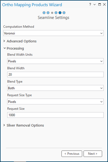
Click Next.
The wizard guided workflow advances to the next pane, Orthomosaic Settings.
Accept all the default settings in the Orthomosaic Settings pane, and click Finish.
The orthomosaic will be generated, listed in the Contents pane, and loaded into the map display.
Summary
In this tutorial, you connected to Server and created a Ortho mapping workspace for drone imagery and used Adjust tools to perform a photogrammetric adjustment with ground control points. You then used tools in the Products group to generate DSM and orthomosaic.
The imagery used in this tutorial was acquired and provided by Esri, Inc.