Local Outlier Analysis (Space Time Pattern Mining Tools)

Summary

Identifies statistically significant clusters and outliers in the context of both space and time. This tool is a space-time implementation of the Anselin Local Moran's I statistic.

Learn more about how the Local Outlier Analysis tool works

Illustration

Usage

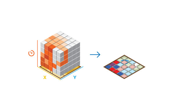
• This tool accepts netCDF files created by various tools in the Space Time Pattern Mining toolbox.

  Learn more about creating a space-time cube

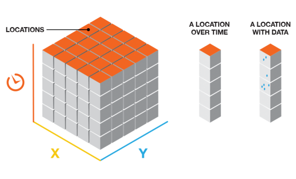
• Each bin in the space-time cube has a LOCATION_ID, time_step_ID, COUNT value, and any Summary Fields or Variables that were included when the cube was created. Bins associated with the same physical location will share the same location ID and together will represent a time series. Bins associated with the same time-step interval will share the same time-step ID and together will comprise a time slice. The count value for each bin reflects the number of incidents or records that occurred at the associated location within the associated time-step interval.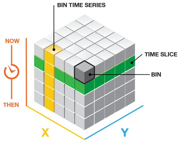

  

• This tool analyzes a variable in the netCDF Input Space Time Cube using a space-time implementation of the Anselin Local Moran's I statistic.

• The Output Features will be added to the Contents pane with rendering that summarizes results of the space-time analysis for all locations analyzed. If you specify a Polygon Analysis Mask, the locations analyzed will be those that fall within the analysis mask; otherwise, the locations analyzed will be those with at least one point for at least one time-step interval.

  

• In addition to the Output Features, an analysis summary is written as messages at the bottom of the Geoprocessing pane when the tool is run. You can access the messages by hovering over the progress bar, clicking the pop-out button , or expanding the details section of the messages in the Geoprocessing pane. You can also access the messages for a previously run tool via Geoprocessing History in the Catalog pane.

• The Local Outlier Analysis tool identifies statistically significant clusters and outliers in the context of both space and time. See How Local Outlier Analysis works for the default output category definitions and additional information about the algorithms used in this analysis tool.

• To identify clusters and outliers in the space-time cube, this tool uses a space-time implementation of the Anselin Local Moran's I statistic, which considers the value for each bin within the context of the values for neighboring bins.

• To determine which bins will be included in each analysis neighborhood, the tool first finds neighboring bins that fall within the specified Conceptualization of Spatial Relationships. Next, for each of those bins, it includes bins at those same locations from N previous time steps, where N is the Neighborhood Time Step value you specify.

• Your choice for the Conceptualization of Spatial Relationships parameter should reflect inherent relationships among the features you are analyzing. The more realistically you can model how features interact with each other in space, the more accurate your results will be. Recommendations are outlined in Selecting a Conceptualization of Spatial Relationships: Best Practices.

• The default Conceptualization of Spatial Relationships is Fixed distance. A bin is considered a neighbor if its centroid falls within the Neighborhood Distance and its time interval is within the Neighborhood Time Step you specify. When you do not provide a Neighborhood Distance value, one is calculated for you based on the spatial distribution of your point data. When you do not provide a Neighborhood Time Step value, the tool uses a default value of 1 time-step interval.

• The Number of Neighbors parameter may override the Neighborhood Distance for the Fixed distance option or extend the neighbor search for the Contiguity edges only and Contiguity edges corners options. In these cases, the Number of Neighbors is used as a minimum number. For instance, if you specify Fixed distance with a Neighborhood Distance of 10 miles and 3 for the Number of Neighbors parameter, all bins will receive a minimum of 3 spatial neighbors even if the Neighborhood Distance has to be increased to find them. The distance is only increased for those bins where the minimum Number of Neighbors is not met. Likewise, with the contiguity options, for bins with fewer than this number of contiguous neighbors, additional neighbors will be chosen based on centroid proximity.

• The Neighborhood Time Step value is the number of time-step intervals to include in the analysis neighborhood. If the time-step interval for your cube is three months, for example, and you specify 2 for the Neighborhood Time Step, all bin counts within the Conceptualization of Spatial Relationships specified, and all of their associated bins for the previous two time-step intervals (covering a nine-month time period) will be included in the analysis neighborhood.

• Permutations are used to determine how likely it would be to find the actual spatial distribution of the values you are analyzing. For each permutation, the neighborhood values around each bin are randomly rearranged and the Anselin Local Moran's I value calculated. The result is a reference distribution of values that is then compared to the actual observed Moran's I to determine the probability that the observed value could be found in the random distribution. The default is 499 permutations; however, the random sample distribution is improved with increasing permutations, which improves the precision of the pseudo p-value.

• If the Number of Permutations parameter is set to 0, the result is a traditional p-value instead of a pseudo p-value.

• The permutations employed by this tool can take advantage of the increased performance available in systems that use multiple CPUs (or multicore CPUs). The tool will default to run using 50 percent of the processors available; however, the number of CPUs used can be increased or decreased using the Parallel Processing Factor environment. The increased processing speed is most noticeable in larger space-time cubes or tool runs with larger numbers of permutations.

• The Polygon Analysis Mask feature layer can include one or more polygons defining the analysis study area. These polygons indicate where point features could possibly occur and should exclude areas where points would be impossible. If you were analyzing residential burglary trends, for example, you might use the Polygon Analysis Mask to exclude a large lake, regional parks, or other areas where there aren't any homes.

• The Polygon Analysis Mask is intersected with the extent of the Input Space Time Cube and will not extend the dimensions of the cube.

• If the Polygon Analysis Mask you are using to set your study area covers an area beyond the extent of the input features that were used when initially creating the cube, you may want to re-create your cube using the Polygon Analysis Mask as the Extent environment. This will ensure that all of the area covered by the Polygon Analysis Mask is included in the Local Outlier Analysis tool. Using Polygon Analysis Mask as the Extent environment setting during cube creation will ensure the extent of the cube matches the extent of the Polygon Analysis Mask.

• This tool creates a new output feature class with the following attributes for each location in the space-time cube. These fields can be used for custom visualization of the output. See How Local Outlier Analysis works for more information about the additional analysis results.

  • Number of Outliers

  • Percentage of Outliers

  • Number of Low Clusters

  • Percentage of Low Clusters

  • Number of Low Outliers

  • Percentage of Low Outliers

  • Number of High Clusters

  • Percentage of High Clusters

  • Number of High Outliers

  • Percentage of High Outliers

  • locations with No Spatial Neighbors

  • locations with an Outlier in the Most Recent Time Step

  • Cluster Outlier Type

  • and additional summary statistics

• The Cluster Outlier Type will always indicate statistically significant clusters and outliers for a 95 percent confidence level, and only statistically significant bins will have values in this field. This significance reflects a False Discovery Rate (FDR) Correction.

• Default rendering for the Output Feature Class is based on the CO_TYPE field and shows locations that were statistically significant. It will show locations that have been part of a significant High-High Cluster, High-Low Outlier, Low-High Outlier, Low-Low Cluster, or classified as Multiple Types over time.

• To ensure at least one temporal neighbor for each location, a Local Moran's Index is not calculated for the first time slice. The bin values in the first time slice are, however, included in the calculation of the global average.

• Running the Local Outlier Analysis tool adds analysis results back to the netCDF Input Space Time Cube. Each bin is analyzed within the context of neighboring bins to measure the clustering for both high and low values and to identify any spatial and temporal outliers within those clusters. The result from this analysis is a Local Moran's I Index, pseudo p-value (or p-value if no permutations were used), and a cluster or outlier type (CO_TYPE) for every bin in the space-time cube.

  A summary of the variables added to the Input Space Time Cube is provided below:

  Variable name	Description	Dimension
  OUTLIER_{ANALYSIS_VARIABLE}_INDEX	The calculated Local Moran's I Index.	Three-dimensions: one Local Moran's I Index value for every bin in the space-time cube.
  OUTLIER_{ANALYSIS_VARIABLE}_PVALUE	Anselin Local Moran's I statistic pseudo p-value or p-value, which measures the statistical significance of the Local Moran's I value.	Three-dimensions: one p-value or pseudo p-value for every bin in the space-time cube.
  OUTLIER_{ANALYSIS_VARIABLE}_TYPE	The result category type distinguishing between a statistically significant cluster of high values (High-High), cluster of low values (Low-Low), outlier in which a high value is surrounded primarily by low values (High-Low), and outlier in which a low value is surrounded primarily by high values (Low-High).	Three-dimensions: one cluster or outlier type for every bin in the space-time cube. The bin is based on an FDR correction.
  OUTLIER_{ANALYSIS_VARIABLE}_HAS_SPATIAL_NEIGHBORS	Indicates locations that have spatial neighbors and those that are relying only on temporal neighbors.	Two-dimensions: one classification for each location. Analysis of locations that do not have spatial neighbors will result in calculations based purely on temporal neighbors.
  OUTLIER_{ANALYSIS_VARIABLE}_ZTRAN	The z-score which is the number of standard deviations that the value deviates from the mean.	Three-dimensions: one z-score value for every bin in the space-time cube.
  OUTLIER_{ANALYSIS_VARIABLE}_LAG	The spatial lag value.	Three-dimensions: one spatial lag value for every bin in the space-time cube.

Parameters

• Dialog
• Python

Label	Explanation	Data type
Input Space Time Cube	The space-time cube containing the variable to be analyzed. Space-time cubes have an .nc file extension and are created using various tools in the Space Time Pattern Mining toolbox.	File
Analysis Variable	The numeric variable in the netCDF file you want to analyze.	String
Output Features	The output feature class containing locations that were considered statistically significant clusters or outliers.	Feature Class
Neighborhood Distance (Optional)	The spatial extent of the analysis neighborhood. This value determines which features are analyzed together to assess local space-time clustering.	Linear Unit
Neighborhood Time Step	The number of time-step intervals to include in the analysis neighborhood. This value determines which features are analyzed together to assess local space-time clustering.	Long
Number of Permutations (Optional)	The number of random permutations for the calculation of pseudo p-values. The default number of permutations is 499. If you choose 0 permutations, the standard p-value is calculated. 0—Permutations are not used and a standard p-value is calculated. 99—With 99 permutations, the smallest possible pseudo p-value is 0.01 and all other pseudo p-values will be even multiples of this value. 199—With 199 permutations, the smallest possible pseudo p-value is 0.005 and all other pseudo p-values will be even multiples of this value. 499—With 499 permutations, the smallest possible pseudo p-value is 0.002 and all other pseudo p-values will be even multiples of this value. 999—With 999 permutations, the smallest possible pseudo p-value is 0.001 and all other pseudo p-values will be even multiples of this value. 9999—With 9999 permutations, the smallest possible pseudo p-value is 0.0001 and all other pseudo p-values will be even multiples of this value.	Long
Polygon Analysis Mask (Optional)	A polygon feature layer with one or more polygons defining the analysis study area. You would use a polygon analysis mask to exclude a large lake from the analysis, for example. Bins defined in the Input Space Time Cube that fall outside of the mask will not be included in the analysis. This parameter is only available for grid cubes.	Feature Layer
Conceptualization of Spatial Relationships (Optional)	Specifies how spatial relationships among features are defined. Fixed distance—Each bin is analyzed within the context of neighboring bins. Neighboring bins inside the specified critical distance (Neighborhood Distance) receive a weight of one and exert influence on computations for the target bin. Neighboring bins outside the critical distance receive a weight of zero and have no influence on a target bin's computations. K nearest neighbors—The closest k bins are included in the analysis for the target bin; k is a specified numeric parameter. Contiguity edges only—Only neighboring bins that share an edge will influence computations for the target polygon bin. Contiguity edges corners—Bins that share an edge or share a node will influence computations for the target polygon bin.	String
Number of Spatial Neighbors (Optional)	An integer specifying either the minimum or the exact number of neighbors to include in calculations for the target bin. For K nearest neighbors, each bin will have exactly this specified number of neighbors. For Fixed distance, each bin will have at least this many neighbors (the Neighborhood Distance will be temporarily extended to ensure this many neighbors if necessary). When one of the contiguity conceptualizations are selected, each bin will be assigned this minimum number of neighbors. For bins with fewer than this number of contiguous neighbors, additional neighbors will be based on feature centroid proximity.	Long
Define Global Window (Optional)	The Anselin Local Moran's I statistic works by comparing a local statistic calculated from the neighbors for each bin to a global value. This parameter can be used to control which bins are used to calculate the global value. Entire cube—Each neighborhood is analyzed in comparison to the entire cube. This is the default. Neighborhood Time Step—Each neighborhood is analyzed in comparison to the bins contained within the specified Neighborhood Time Step. Individual time step—Each neighborhood is analyzed in comparison to the bins in the same time step.	String

Environments

Current Workspace, Scratch Workspace, Output Coordinate System, Geographic Transformations, Random number generator, Parallel Processing Factor

Special cases

Random number generator

The Random Generator Type used is always Mersenne Twister.

Licensing information

• Basic: Yes
• Standard: Yes
• Advanced: Yes

Related topics

• An overview of the Space Time Pattern Analysis toolset
• How Local Outlier Analysis works
• Create Space Time Cube By Aggregating Points
• Visualize the space-time cube
• What is a z-score? What is a p-value?
• An overview of the Space Time Pattern Mining toolbox
• How Cluster and Outlier Analysis (Anselin Local Moran's I) works
• Find a geoprocessing tool