Compare Neighborhood Conceptualizations (Spatial Statistics Tools)

Summary

Selects the spatial weights matrix (SWM) from a set of candidate SWMs that best represents the spatial patterns (such as trends or clusters) of one or more numeric fields.

The output spatial weights matrix file can then be used in tools that allow .swm files for their Neighborhood Type or Conceptualization of Spatial Relationships parameter values, such as the Bivariate Spatial Association (Lee's L), Hot Spot Analysis (Getis-Ord Gi*), and Cluster and Outlier Analysis (Anselin Local Moran's I) tools.

The tool selects the SWM by creating spatial components (called Moran eigenvectors) from each candidate SWM and testing how effectively the components represent the spatial patterns of the input fields.

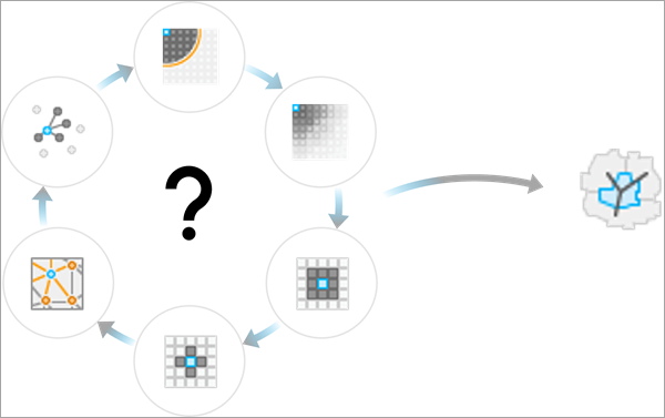
Learn more about Moran eigenvectors

Illustration

Compare Neighborhood Conceptualizations tool illustration

Usage

The purpose of the tool is to suggest a neighborhood type and weighting scheme (sometimes called a conceptualization of spatial relationships) that best represent the spatial patterns of the input fields by testing which spatial weighting produces spatial components that can most accurately predict the values of the input fields. The reasoning is that each spatial component has a spatial pattern, and the components that can most accurately predict the input fields are those that have the most similar patterns to the input fields. However, this suggested SWM is not intended to be a replacement for individual or expert knowledge of the data and its processes. There are many considerations to make when choosing a SWM for an analysis, and this tool only uses the ability of the spatial components to predict the input fields to determine the suggested SWM. In some cases, such as with the Hot Spot Analysis (Getis-Ord Gi*) tool, there are alternative methodologies for choosing a SWM, such as using the distance band that maximizes the spatial autocorrelation of the data (this is how the Optimized Hot Spot Analysis tool determines its neighbors and weights). It is recommended that you try alternative methodologies for neighborhoods and spatial weights and use the method that best aligns with the goals of the analysis.
Provide all the fields to the Input Fields parameter that you will use in any subsequent analysis using the output .swm file. For example, the Hot Spot Analysis (Getis-Ord Gi*) tool only requires one field, but the Bivariate Spatial Association (Lee's L) tool requires two fields. You can provide the output .swm file in the Weights Matrix File parameter after specifying the Get spatial weights from file option for the Neighborhood Type or Conceptualization of Spatial Relationships parameter of subsequent analysis tools.
The geoprocessing messages include the Neighborhood Search History table that displays details of each tested SWM (such as the number of neighbors and weighting scheme) and the adjusted R-squared value of the SWM when used to predict the input fields. The SWM suggested by the tool will be the one with the largest adjusted R-squared and will be indicated by bold text and an asterisk in the table.
To select the SWM, the tool generates a list of candidate SWMs and tests which one creates spatial components that best represent the spatial patterns of the input fields. If no SWMs are provided in the Input Spatial Weights Matrix Files parameter, 28 SWMs will be created and included in the candidate list (see Understanding Moran eigenvectors for descriptions of each SWM). If any input SWMs are provided, you can use the Compare Only Input Spatial Weight Matrices parameter to choose whether the candidate list only includes the provided SWMs or whether the candidate list includes the provided SWMs and the 28 SWMs created by the tool. For example, to use a single specified SWM, provide the SWM in the Input Spatial Weights Matrix Files parameter and leave the Compare Only Input Spatial Weight Matrices parameter checked.
The tool determines the suggested SWM using the following procedure:
1. For each SWM, the Moran eigenvectors with the largest eigenvalues (those with the strongest autocorrelation) are generated. The number of eigenvectors is equal to 25 percent of the number of features, up to a maximum of 100.
2. Any eigenvectors that have negative Moran's I values (meaning that they are negatively autocorrelated) are filtered out.
3. Each input field is predicted individually using the eigenvectors as explanatory variables in an ordinary least-squares regression model.
4. The total sum of squares and residual sum of squares for all fields are aggregated, and a combined adjusted R-squared value is calculated.
5. The SWM with the highest adjusted R-squared value is returned.
This procedure is fully described in the following reference:
- Bauman, David, Thomas Drouet, Marie-Josée Fortin, and Stéphane Dray. 2018. "Optimizing the choice of a spatial weighting matrix in eigenvector-based methods." Ecology 99, no. 10: 2159-2166. https://doi.org/10.1002/ecy.2469.

Label	Explanation	Data type
Input Features	The input features containing the fields that will be used to select the SWM.	Feature Layer
Input Fields	The input fields that will be used to select the SWM.	Field
Output Spatial Weights Matrix	The output `.swm` file of the neighbors and weights selected by the tool.	File
Unique ID Field	The unique ID field of the output `.swm` file. The field must be an integer and must have a unique value for each input feature.	Field
Input Spatial Weights Matrix Files (Optional)	The input `.swm` files that will be used as candidates for the SWM that best represents the spatial patterns (such as trends or clusters) of one or more numeric fields. If no files are provided, the tool will test 28 different neighborhoods.	File
Compare Only Input Spatial Weight Matrices (Optional)	Specifies whether only the `.swm` files provided in the Input Spatial Weights Matrix Files parameter will be tested or whether 28 additional neighborhoods will also be tested. The tool will use the SWM that creates spatial components that best represents the spatial patterns (such as trends or clusters) of one or more numeric fields. This parameter only applies if at least one input `.swm` file is provided. Checked—Only the input `.swm` files provided in the `in_swm` parameter will be tested. This is the default. Unchecked—The input `.swm` files provided in the `in_swm` parameter and an additional 28 neighborhoods will be tested.	Boolean

arcpy.stats.CompareNeighborhoodConceptualizations(in_features, input_fields, out_swm, id_field, {in_swm}, {compare_only_inputs})

Name	Explanation	Data type
in_features	The input features containing the fields that will be used to select the SWM.	Feature Layer
input_fields [input_fields,...]	The input fields that will be used to select the SWM.	Field
out_swm	The output `.swm` file of the neighbors and weights selected by the tool.	File
id_field	The unique ID field of the output `.swm` file. The field must be an integer and must have a unique value for each input feature.	Field
in_swm [in_swm,...] (Optional)	The input `.swm` files that will be used as candidates for the SWM that best represents the spatial patterns (such as trends or clusters) of one or more numeric fields. If no files are provided, the tool will test 28 different neighborhoods.	File
compare_only_inputs (Optional)	Specifies whether only the `.swm` files provided in the `in_swm` parameter will be tested or whether 28 additional neighborhoods will also be tested. The tool will use the SWM that creates spatial components that best represents the spatial patterns (such as trends or clusters) of one or more numeric fields. This parameter only applies if at least one input `.swm` file is provided. `COMPARE_INPUTS`—Only the input `.swm` files provided in the `in_swm` parameter will be tested. This is the default. `COMPARE_ALL`—The input `.swm` files provided in the `in_swm` parameter and an additional 28 neighborhoods will be tested.	Boolean

Code sample

CompareNeighborhoodConceptualizations example 1 (Python window)

The following Python window script demonstrates how to use the CompareNeighborhoodConceptualizations function:

# Select the spatial weights matrix (SWM) that best describes the
# spatial patterns of POP_SQMI.

arcpy.env.workspace = r"c:\data\project_data.gdb"

arcpy.stats.CompareNeighborhoodConceptualizations(
    in_features="states",
    input_fields="POP_SQMI",
    out_swm=r"c:\data\states.swm",
    id_field="unique_id_field"
)

CompareNeighborhoodConceptualizations example 2 (stand-alone script)

The following stand-alone script demonstrates how to use the CompareNeighborhoodConceptualizations function:

# Select the spatial weights matrix (SWM) that best describes
# the spatial patterns of two analysis field.

import arcpy

# Set the current workspace.
arcpy.env.workspace = r"c:\data\project_data.gdb"

# Run the tool.
arcpy.stats.CompareNeighborhoodConceptualizations(
    in_features="myFeatureClass",
    input_fields="myAnalysisField1;myAnalysis Field2",
    out_swm=r"myOutputSWM.swm",
    id_field="myUniqueIDField"
)

# Print the tool messages.
print(arcpy.GetMessages())

Environments

This tool does not use any geoprocessing environments.

Licensing information

Basic: Yes
Standard: Yes
Advanced: Yes