How Evaluate Bin Sizes for Point Aggregation works
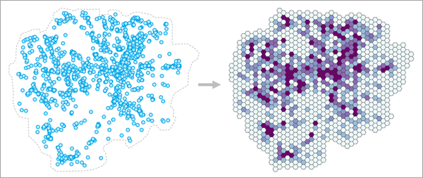
The Evaluate Bin Sizes for Point Aggregation tool helps you choose an appropriate bin size when aggregating points into square or hexagon bins arranged in a tessellation. The tool also allows you to assess various other bin sizes to determine how the resulting patterns would change if other bin sizes were used instead. You can choose to aggregate point counts into bins (such as counting emergency calls) or average the values of a numeric field (such as average home sale price) within each bin.
Aggregating points within bins is a common workflow in GIS, including aggregating emergency calls, service outages, and temperatures. It is also used to better visualize large blobs of points and to protect privacy by obscuring individual point locations and values. However, despite the many applications, there is relatively little guidance on how large these bins should be. In practice, bin sizes are often chosen by convenience (for example, using a round number) or choosing whichever bin size produces results that are most visually pleasing. However, the choice of scale changes both what you can detect and how you interpret it (an example of the modifiable areal unit problem), so it is important to make defensible and reproducible decisions. It is also important to characterize how sensitive the results are to the bin size: would using a larger or smaller bin size lead to different patterns and conclusions?
Fundamentally, determining an appropriate bin size for aggregating point data into bins is a scale problem. Bins that are too small will have erratic values with many bins having no points, and bins that are too large will blur away and mask important local patterns. An appropriate bin size is one that is large enough to produce a wide variety of stable values but still small enough that local patterns of points are preserved in the resulting bins (rather than being aggregated away).
To determine an appropriate bin size, a range of candidate bin sizes are evaluated using two criteria: one that prefers smaller bin sizes and one that prefers larger bin sizes.
These two metrics (each a value between 0 and 1) are then multiplied together to produce a single evaluation score for each bin size, and the bin size with the highest evaluation score is recommended by the tool. The evaluation score curve also allows you to see how other bin sizes compared to the bin size recommended by the tool.
See the Bin size evaluation additional details section below for more information about evaluation scores and how they are calculated.
Define an appropriate aggregation boundary
In addition to providing the points that will be aggregated, you must also use the Aggregation Boundary parameter to define the area in which the points will be aggregated and bins will be created. The aggregation boundary (sometimes called a study area or area of interest) should define the area where points can occur and be recorded. For example, when aggregating emergency calls within a city, the city boundary should be used as the aggregation boundary because an emergency call can come from anywhere within the city, and any call from outside the city would not be included in the dataset. While it is tempting to think of the bins being created and then clipped to the aggregation boundary, the boundary instead has a deep impact on the evaluation scores and the recommended bin size. Choosing an inappropriate aggregation boundary often causes unrealistically large or small recommended bin sizes, so it is strongly recommended that you consider which boundary is most appropriate for your data.
Providing a boundary to delineate where points can and cannot occur is important because the tool must be able to differentiate whether an area has no points because it happened to have no incidents (such as a section of a city having no robberies in a particular week) or whether it is not possible for points to be observed in the area (such as whale sightings on the land). Because the tool assesses the variety of the resulting point counts of the bins, counts equal to zero are just as important as any other counts, and the tool will avoid bin sizes that result in a large proportion of bins with no points. In practice, this means that if the aggregation boundary is too large (meaning that it contains many areas where points cannot be recorded), the recommended bin size will be unrealistically large in order fill in the gaps and reduce the number of empty bins. Conversely, if the study area is too small, the tool will recommend smaller bin sizes to increase the number of bins with no points.
Note:
If an analysis field is provided, the aggregation boundary must still be provided, but it is less important for estimating an appropriate bin size. This is because analysis field averages can only be calculated for bins that contain at least one point, so any bin with no points will not be used to estimate the bin size.
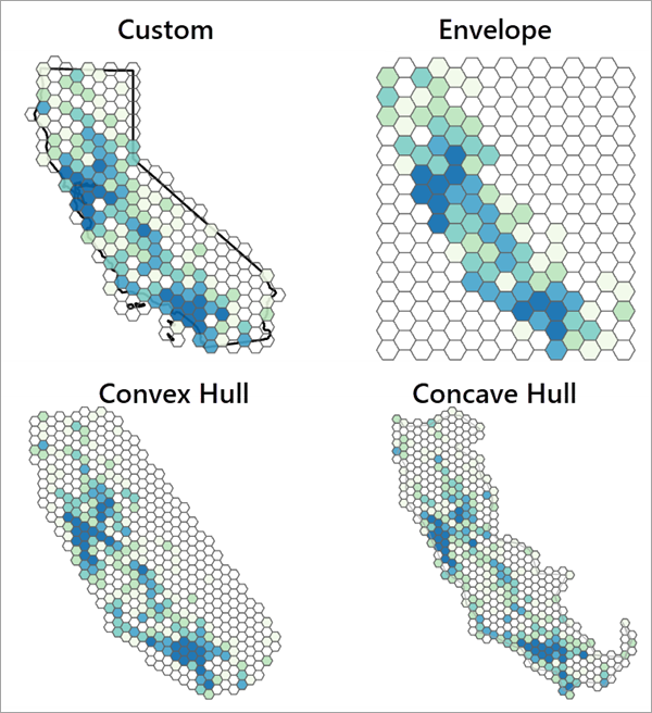
If an appropriate aggregation boundary for the points is known (such as the boundary of a city), choose the Custom polygons option and provide the boundary in the Custom Polygons parameter. You can also draw the aggregation boundary polygon using interactive feature input.
If an appropriate aggregation boundary is not known, the boundary can be automatically created using the Concave hull, Convex hull, or Envelope options (see Minimum Bounding Geometry for more information). When using an automatically created boundary, you should always visually assess whether the boundary adequately represents the points. If the boundary is inappropriate, use a different option or interactively draw a boundary that better represents the points.
The following image shows the resulting bin sizes for the same data using all options of the Aggregation Boundary parameter. The custom option uses the actual boundary in which the points were collected. For other datasets (and especially those with spatial outliers), the difference in resulting bin sizes and patterns can be even more extreme.
Aggregate in space and time
If the points have a date-time field indicating the time that each point was recorded, you can use the Time Field and Time Interval parameters to aggregate the points in space and time. For example, for points representing emergency calls over the course of a year that you wish to aggregate each week, the tool will recommend a single bin size that is most appropriate to reuse for every week of the year. This is especially useful when you intend to aggregate the points into a space-time cube.
To estimate the bin size, the data will be separated into different time intervals, starting at the latest time field value and going backwards in time. For example, if the data spans an entire year, and you use a one week time interval, all data in the final week of the year will be in the same time interval; all data in the seven prior days will be in the same time interval; and so on. Any point whose time field value occurs on the boundary between two time intervals will be included in the earlier interval.
For each tested bin size, bins will be created separately in each time interval, and the resulting point counts or analysis variable means will be combined together across all time intervals before calculating the evaluation scores. For example, if there are 10 time intervals with 50 bins in each interval, then the evaluation score for the bin size will be calculated using 500 bin values. The recommended bin size will be the one that best balances the metrics through the entire time range of the data.
Splitting the points into time intervals often results in the earliest time interval being incomplete, such as one day being left over when aggregating yearly data into weekly time intervals. To prevent the incomplete interval with few points from biasing the recommended bin size, the earliest time interval will be not be used to estimate the bin size if it contains fewer points than every other time interval. Even if the earliest time interval is not used to estimate the bin size, bins will still be created for every time interval in the output feature class.
Tool outputs
The tool creates three outputs that are contained in a group layer. The primary output is a polygon feature class of the aggregated bins using the recommended bin size. The layer is symbolized by the point count or analysis field mean within each bin. If a time field is provided, the feature class will be time-enabled with separate polygon bins for each time interval (in the output layer, the bins of different time intervals will draw on top of each other).
The second output is a polygon feature class of the aggregation boundary that was used by the tool. This output is most useful for the concave and convex hull options in order to see the shapes of the boundaries. The third output is a table containing the evaluation scores for all bin sizes tested by the tool. The table comes with charts that can be used to investigate the bin sizes.
Evaluation Scores Across Bin Sizes chart
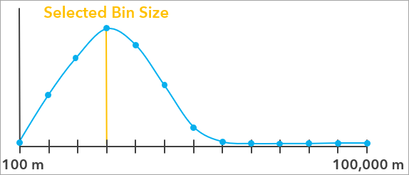
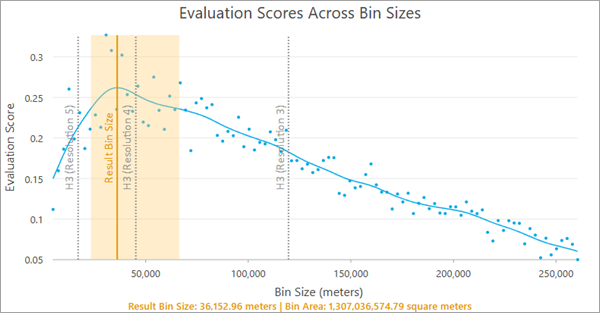
The Evaluation Scores Across Bin Sizes chart displays the evaluation scores for all tested bin sizes. The blue points in the chart are the raw evaluation scores for the bin sizes, and they are smoothed with a spline (the blue curve). The largest value of the blue curve is the recommended bin size and is indicated by a vertical orange line. A light orange confidence region is also displayed around the recommended bin size, and any bin size in this range has an evaluation score that is not significantly lower than the recommended bin size, so you can choose any value in this range (for example, choosing a round number) without a significant decrease to the evaluation score.
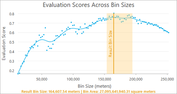
The recommended bin size and the associated area of each bin are displayed at the bottom of the chart. For square bins, the bin size is the width or height of each square, and for hexagons, the bin size is the height of each hexagon (the distance from one flat edge to the opposite flat edge). If a time field and time interval are provided, the time interval will also be displayed.
Note:
The smallest bin size tested (the minimum value of the x-axis) is the bin size that results in 20 bins for every input point (in other words, the bins are so small that more than 95 percent of them will contain no points), and the largest bin size (the maximum value of the x-axis) is 25 percent of the x- or y-extent of the aggregation boundary, whichever is larger. The tool tests 100 bin sizes evenly incremented between the minimum and maximum.
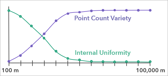
Internal Uniformity and Point Count Variety Across Bin Sizes chart
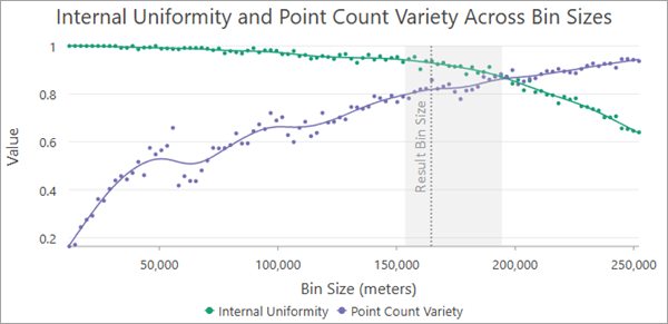
When aggregating point counts without an analysis field, the Internal Uniformity and Point Count Variety Across Bin Sizes chart displays the two criteria that were combined together to produce the evaluation scores. For each tested bin size, a green curve displays the internal uniformity score, and a purple curve shows the point count variety score. Usually, the green curve will decrease and the purple curve will increase. The recommended bin size and the confidence interval are also displayed for context. The recommended bin size will generally have reasonable scores for both criteria, indicating an effective balance between the opposing criteria. See the Bin size evaluation additional details section below for more information about each criteria.
Internal Uniformity and Variance Loss Across Bin Sizes chart
When averaging the values of an analysis field, the point count variety metric is replaced with a variance loss metric. Like point count variety, it usually prefers larger bin sizes and attempts to produce bin averages with as much variability and variety as possible. See the Bin size evaluation additional details section below for more information about the variance loss metric.
Geoprocessing messages
The messages of the tool include various sections summarizing the input points and the resulting bins. The information includes the recommended bin size, summary statistics of the resulting bin counts or analysis field averages, and information about the aggregation boundary. If a time field is provided, information about the time intervals is also provided.
Note:
The statistics shown in the messages will be calculated only from the values that are used to estimate the evaluation scores. If you combine coincident points or the earliest time interval is excluded, some statistics (such as the standard deviation of the analysis field) will be different than the values of the original points.
Best practices and limitations
The following are best practices and limitations when using the tool:
The tool assumes that there is a single bin size that is appropriate for aggregating the points. However, in many cases, there is no single bin size that will adequately represent the points across the entire aggregation boundary. For example, in a large county that has rural areas with low population density and urban areas with high population density, it may be difficult to aggregate emergency calls across the entire county. Bins small enough to adequately represent the urban areas will be mostly empty in rural areas, while bins large enough for rural areas will condense urban centers into only a few bins. A common sign of this problem is very wide confidence intervals around the recommended bin size, indicating high uncertainty about which bin size to use. A potential solution is to separate the points into different datasets and aggregate them separately using different bin sizes.
The tool is most appropriate when you intend to perform some kind of analysis using the resulting point counts (for example, hot spot analysis or local outlier analysis) rather than simple cartographic smoothing. While it can be effective to smooth large blobs of points for better visual representation, the primary purpose of the tool is to produce aggregated bins that best maintain the spatial structure of the points and produce values that are conducive to analysis.
Large numbers of coincident points (multiple points at the same coordinate) can produce unrealistic bin sizes. The tool will return a warning if any of the input points are coincident. If time intervals are used, coincident points will be detected within each time interval independently. If you provide an analysis field, you can use the Combine Coincident Points parameter to average the values of coincident points before evaluating the bin sizes.
Bin size evaluation additional details
The general methodology of the tool is to evaluate a range of bin sizes using two metrics. When counting points, the metrics are internal uniformity and point count variety, and when averaging the values of an analysis field, the metrics are internal uniformity and variance loss. Each bin size is given a score between 0 and 1 for each metric, and the values are multiplied together to produce a final evaluation score that balances both criteria. The internal uniformity metric generally prefers smaller bin sizes, whereas the point count variety and variance loss metrics generally prefers larger bin sizes, so bin sizes with the highest evaluation scores are those in the middle that best compromise between the opposing criteria. The following sections further describe the criteria.
Internal uniformity
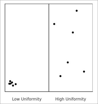
The internal uniformity metric measures whether the points are uniformly distributed within the resulting bins. For example, in the image below, the points in the bin on the left are highly clustered in a corner, but the points are randomly and uniformly scattered throughout the bin on the right, so the bin on the right has higher internal uniformity.
Internal uniformity is important in order to avoid choosing a bin size that hides important local patterns. If the points within a bin form a strong cluster or pattern, summarizing them with a single count or average may be misleading. This metric checks whether the points within each bin are randomly arranged, which suggests the bin is a fair and representative summary of the points inside it. When many bins show structured patterns, it is a sign that the bin size may be too large, hiding important patterns within the bins.
The metric is calculated by testing the point locations for complete spatial randomness, and the value is the proportion of bins with a p-value greater than 0.05 (meaning that they were not detected to be clustered). Bins with no points are not included in the proportion because empty cells cannot be classified as spatially random or clustered.
The test for complete spatial randomness divides each bin into a number of smaller bins. For squares, the bin is divided into 25 smaller squares, and for hexagons, the bin is divided into 24 triangles. The counts of points within the squares or triangles are then tested for uniformity using a chi-square goodness of fit test.
Point count variety
The point count variety metric quantifies the diversity of point counts across bins and favors bin sizes that result in a wide variety of count values, avoiding bin sizes that have large proportions of empty bins along with a small number of bins with large counts. Conceptually, this encourages informational richness, reflecting the idea that aggregations should produce meaningful variation and diversity in the point counts, which is particularly desirable when you intend to perform an analysis (such as hot spot analysis) on the point counts. In practice, this metric tends to increase with bin size, as larger bins tend to accumulate more diverse and evenly distributed counts.
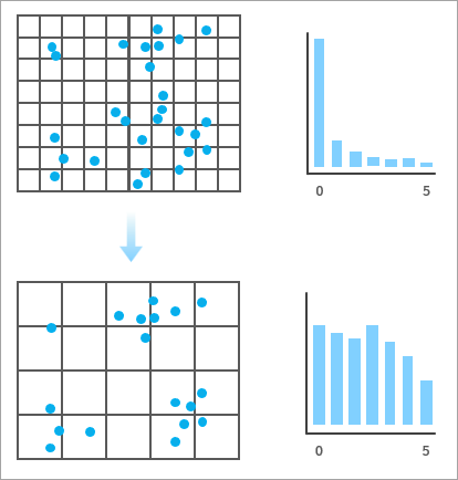
For example, in the image below, the bins on the bottom produce a wider variety and more even distribution of point counts than the bins on the top, so the bottom bins would receive a higher score for point count variety. In general, the closer the distribution of point counts is to a uniform (flat) distribution, the higher the score.
The metric is calculated using a normalized Shannon entropy measure. For each bin size, the distribution of bin counts is divided into five equal intervals, and the entropy of this distribution is calculated. This entropy is then divided by the entropy of a uniform distribution, producing a score between 0 and 1.
Note:
When an analysis field is not used, the internal uniformity and point count variety scores are generated by simulating random squares or hexagons within the aggregation boundary rather than constructing a full tessellation for each bin size. This improves processing speed, but results will be slightly different when rerunning the tool. However, you can use the Random Number Generator environment to ensure reproducible results. The number of simulated polygons for each bin size is calculated such that 75 percent of the aggregation boundary is covered by the simulations, on average.
Variance loss
The variance loss metric quantifies how much of the variance of the original analysis field values is preserved in the bin averages. The metric is calculated with the following formula:
In the formula, \(Var_w(\bar{X_b})\) is the weighted variance of the bin averages (weighted by the number of points in each bin), and \(Var(X)\) is the variance of the original analysis field.
This metric measures how quickly the variance of the bin means decreases as the bin size increases and attempts to preserve as much variability of the original analysis field as possible. The variance ratio is subtracted from one so that it produces larger scores for larger bin sizes yet still captures how the variance loss scales with increasing bin size.
Note:
When an analysis field is used, the internal uniformity and variance loss scores are also estimated using simulated bins. However, each simulated bin must contain at least one point in order to be included. For each tested bin size, the tool will attempt 1000 simulated bins, and if fewer than 100 simulations contain a point, the bin size will be skipped and not receive evaluation scores. The number of valid samples is saved as a field in the output table.
Bootstrapped confidence intervals
The orange confidence intervals around the recommended bin size in the charts are constructed using bootstrapping. This process randomly resamples the evaluation scores with replacement and estimates a spline for each resampled set of evaluation scores. For each resampling, the evaluation score of the original recommended bin size is recorded, and the fifth percentile is determined. Any bin size whose evaluation score is above this value will be included in the confidence interval. These bin sizes can be interpreted as having evaluation scores that are not significantly lower than the evaluation score of the bin size recommended by the tool.
H3 hexagons
The tool does not allow aggregation into H3 hexagons. However, when aggregating into hexagons, you can display the associated H3 resolutions as guides in the Evaluation Scores Across Bin Sizes chart. By default, the guides are disabled, but you can enable them on the Guides tab of the Chart Properties pane.
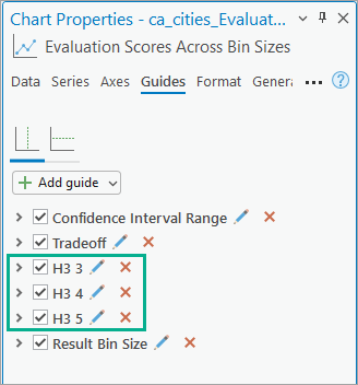
When enabled, the guides (dashed vertical gray lines) allow you to see the evaluation scores of the H3 resolutions that are within the range of tested bin sizes and choose the best one for your data. For example, in the image below, H3 resolution 4 has the highest evaluation score, is closest to the recommended bin size, and is within the confidence interval.
References
The following resources were used to implement the tool:
- Ramos, Rafael G. 2025. "Finding an Adequate Areal Unit to Map Crime: A Spatial Data Perspective." New Research in Crime Modeling and Mapping Using Geospatial Technologies (pp. 27-44). Cham: Springer Nature Switzerland. https://doi.org/10.1007/978-3-031-81580-5_2.