IDW 3D (Geostatistical Analyst Tools)

Summary

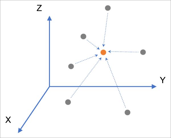
Interpolates the values of 3D points using inverse distance weighting (IDW) and creates a voxel layer and source file (.nc) of the predicted values.

Illustration

Usage

• Compared to the Empirical Bayesian Kriging 3D (EBK 3D) tool that also performs 3D interpolation, IDW 3D is a faster and simpler tool in which no assumptions about the distribution or trends of the data values are made. IDW 3D is an exact interpolation method, meaning that the 3D prediction surface will pass through the measured values of input points exactly, making it a useful visualization tool for irregular 3D points.

  IDW 3D generally produces less accurate predictions than EBK 3D, and it is particularly sensitive to clustered input points. IDW 3D cannot produce standard errors of predicted values, so estimation of the uncertainty of the predictions is not supported.

• The tool predicts values at each new location in 3D using a weighted average of the values of the input points that are within the 3D search neighborhood of the prediction location. The weight for each neighboring point is the inverse distance (one divided by the distance) to the prediction location, taken to a power (exponent). The weights are normalized to sum to 1 in the weighted average.

  Learn more about IDW

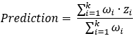  • , where k is the number of neighbors, ω_i is the weight of neighbor i, and z_i is the measured value of neighbor i.

  • , where d_i is the 3D Euclidean distance to the prediction location for neighbor i, and p is the power value.

• If the tool is run in a local scene with the same horizontal and vertical coordinate systems as the input features, a voxel layer will be added to the scene allowing you to interactively explore the results. You can also add the output netCDF file as a voxel layer using the Make Multidimensional Voxel Layer tool or the Add Multidimensional Voxel Layer dialog box.

  You can convert the output netCDF file to a multidimensional raster using the Copy Raster tool. You can also add it to a map as a feature or raster layer using the Make NetCDF Feature Layer tool or Make NetCDF Raster Layer tool, respectively.

• Summary statistics based on leave-one-out cross validation are displayed as geoprocessing messages to assess the accuracy and reliability of the predictions. The following summary statistics are displayed:

  • Count—The number of features with cross validation results. This value can be different than the number of the input features when some features have null values, have coincident locations, or are unable to locate neighboring features.

  • Mean Error—The average of the cross validation errors. This statistic measures model bias and should be as close to zero as possible. Positive values indicate a tendency to overpredict (predict values that are larger than the measured values), and negative values indicate a tendency to underpredict.

  • Root Mean Square Error—The square root of the average squared cross validation errors. This statistic measures prediction accuracy and should be as small as possible. The value estimates the average difference between the predicted values and the measured values. For example, for temperature interpolation in degrees Celsius, a root mean square error value of 1.5 means that the predictions are expected to differ from the true values by approximately 1.5 degrees, on average.

  Learn more about cross validation

• The input features must be 3D points with elevations stored in the Shape.Z geometry attribute. You can convert 2D point features with an elevation field into 3D point features using the Feature To 3D By Attribute tool.

  It is recommended that the input features have a vertical coordinate system that accurately defines their z-coordinates. You can assign a vertical coordinate system to the points using the Define Projection tool.

• Use the Output cross validation feature class parameter to investigate the cross validation errors of each input point. The measured values and cross validation predictions are stored as fields on the feature class.

  The feature class will contain two scatter plots to investigate trends in the cross validation results:

  • Cross Validation: Predicted versus Measured—Displays the cross validation predictions versus the measured values. If the predicted values are approximately equal to the measured values (indicating accurate interpolation results), the points in the scatter plot should form a line with a slope equal to 1.

  • Cross Validation: Measured versus Error—Displays the measured values versus the cross validation errors. If the errors are independent of the measured values, the points in the scatter plot will show no patterns or trends, and the trend line will be flat (slope approximately equal to 0). Trend lines with a negative slope (decreasing) indicate a smoothing effect in the interpolation model, meaning that the model has a tendency to underpredict large values and overpredict small values.

  Learn more about interpreting cross validation charts

• The input features and the minimum and maximum elevation clipping rasters must be in a projected coordinate system. If the points or rasters have a geographic coordinate system with latitude and longitude coordinates, they must be projected to a projected coordinate system using the Project or Project Raster tool.

• When laying out the 3D grid of points that will represent the voxels, the first point is created at the minimum x-, minimum y-, and minimum z-coordinate of the output extent (by default, the extent of the input features). The remaining points are created by iterating the X spacing, Y spacing, and Elevation spacing parameter distances through the dimensions of the output extent. If any of the spacing distances do not evenly divide the corresponding dimension of the output extent, one row or column of points will be created beyond the output extent. For example, if the output extent for x is specified as 0 through 10 and the X spacing parameter is specified as 3, the output will have five rows in the x-extent: 0, 3, 6, 9, and 12. Similarly, an additional row or column of points will be created if the spacing distances do not evenly divide the y- or z-extents.

• The Input study area polygons, Minimum elevation clipping raster, and Maximum elevation clipping raster parameters can be used to limit the analysis within a specific study area and between two elevation surfaces. Any voxels outside these bounds will have no value and will not display. For example, if the points are located within a marine preserve, you can create a voxel layer that displays only within a polygon of the preserve (study area), above the ocean floor (minimum elevation raster), and below the thermocline (maximum elevation raster).

  There are various considerations for using elevation surfaces as minimum or maximum elevation rasters. Image services, web elevation layers, and web imagery layers will have the slowest performance and errors may occur for large numbers of queries. Rasters saved as local files on disk will have the fastest performance and are recommended when creating high-resolution voxel layers over large spatial extents.

• If the input features have a selection, the values of the X spacing, Y spacing, and Elevation spacing parameters will recalculate while the tool is running based on the extent of the selected features. The recalculated values will print as warning messages when the tool completes. If you manually provide a value for a spacing parameter (or provide an output extent), the value will not recalculate.

• If input study area polygons are provided, the extent of the study area will be used as the default output extent, and the X spacing and Y spacing parameter values will recalculate based on this extent. This ensures that the output will fill the entirety of the study area by default.

Parameters

• Dialog
• Python

Label	Explanation	Data type
Input features	The 3D point features that contain the field that will be interpolated. The points must be in a projected coordinate system.	Feature Layer
Value field	The field from the input features containing the measured values that will be interpolated.	Field
Output netCDF file	The output netCDF file that will contain the predicted values in a 3D grid. This file can be used as the data source of a voxel layer.	File
Power (Optional)	The power value that will be used to weight the values of neighboring features when calculating predictions. A higher power results in higher influence to closer points. The value must be between 1 and 100. The default is 2.	Double
Elevation inflation factor (Optional)	A constant value that is multiplied to the z-coordinates of the input features prior to finding neighbors and calculating distances. For most 3D data, the values of the points change faster vertically than horizontally, and this factor stretches the locations of the points so that one unit of distance vertically is equivalent to one unit of distance horizontally. The locations of the points will be moved back to their original locations before returning the result of the interpolation. If no value is provided, one will be estimated while the tool runs and will be displayed as a geoprocessing message. The estimated value is determined by minimizing the root mean square cross validation error. The value must be between 1 and 1,000.	Double
Output cross validation feature class (Optional)	A feature class of the cross validation statistics for each input point. The feature class will contain two scatter plots.	Feature Class
X spacing (Optional)	The spacing between each gridded point in the x-dimension. The default value creates 40 points along the output x-extent.	Linear Unit
Y spacing (Optional)	The spacing between each gridded point in the y-dimension. The default value creates 40 points along the output y-extent.	Linear Unit
Elevation spacing (Optional)	The spacing between each gridded point in the elevation (z) dimension. The default value creates 40 points along the output z-extent.	Linear Unit
Input study area polygons (Optional)	The polygon features that represent the study area. Only points that are within the study area are saved in the output netCDF file. When visualized as a voxel layer, only voxels within the study area will display in the scene. Points are determined to be inside or outside the study area using only their x- and y-coordinates.	Feature Layer
Minimum elevation clipping raster (Optional)	The elevation raster that will be used to clip the bottom of the voxel layer. Only voxels above this elevation raster will be assigned predictions. For example, if you use a ground elevation raster, the voxel layer will only display above the ground. It can also be used for bedrock surfaces or the bottom of a shale deposit. The raster must be in a projected coordinate system, and the elevation values must be in the same unit as the vertical unit of the raster.	Raster Layer
Maximum elevation clipping raster (Optional)	The elevation raster that will be used to clip the top of the voxel layer. Only voxels below this elevation raster will be assigned predictions. For example, if you use a ground elevation raster, the voxel layer will only display below the ground. It can also be used to clip voxels to the top of a restricted airspace. The raster must be in a projected coordinate system, and the elevation values must be in the same unit as the vertical unit of the raster.	Raster Layer
Search neighborhood (Optional)	Specifies the number and orientation of the neighbors that will be used to predict values at new locations. Standard3D Max neighbors—The maximum number of neighbors per sector that will be used to estimate the value at the unknown location. Min neighbors—The minimum number of neighbors per sector that will be used to estimate the value at the unknown location. Sector type—The geometry of the 3D neighborhood. Sectors are used to ensure that neighbors are used in every direction around the prediction location. All sector types are formed from the Platonic solids. 1 Sector (Sphere)—The closest neighbors from any direction will be used. 4 Sector (Tetrahedron)—Space will be divided into 4 regions, and neighbors will be used in each of the 4 regions. 6 Sector (Cube)—Space will be divided into 6 regions, and neighbors will be used in each of the 6 regions. 8 Sector (Octahedron)—Space will be divided into 8 regions, and neighbors will be used in each of the 8 regions. 12 Sector (Dodecahedron)—Space will be divided into 12 regions, and neighbors will be used in each of the 12 regions. 20 Sector (Icosahedron)—Space will be divided into 20 regions, and neighbors will be used in each of the 20 regions. Radius—The length of the radius of the search neighborhood. If no value is provided, a value will be estimated while the tool runs, and the estimated value will be displayed as a geoprocessing message.	Geostatistical Search Neighborhood

Derived output

Label	Explanation	Data type
Count	The total number of samples used.	Long
Mean error	The averaged difference between the measured and the predicted values.	Double
Root mean square	Indicates how closely the model predicts the measured values.	Double
Output voxel layer	A voxel layer of the predicted values.	Voxel Layer

Environments

Coincident Points, Extent, Parallel Processing Factor

Licensing information

• Basic: Requires Geostatistical Analyst
• Standard: Requires Geostatistical Analyst
• Advanced: Requires Geostatistical Analyst

Related topics

• An overview of the Interpolation toolset
• Find a geoprocessing tool